Skip to content

Archive for

#95 Independence day, part 1

One of my favorite class sessions when I teach probability is the day that we study independent events.  This post will feature questions that I pose to students on this topic, which (as usual) appear in italics.


I introduce conditional probability and independence with some real data that Beth Chance and I collected in 1998, when the America Film Institute unveiled a list of what they considered the top 100 American films (see the list here).  Beth and I tallied up which films we had seen and produced the following table of counts:

Suppose that one of these 100 films is selected at random, meaning that each of the 100 films is equally likely to be selected.

  • a) What is the probability that Beth has seen the film?
  • b) Given the partial information that Allan has seen the film, what is the updated (conditional) probability that Beth has seen it?
  • c) Does learning that Allan has seen the randomly selected film change the probability that Beth has seen it?  In which direction?  Why might this make sense?
  • d) Repeat this analysis based on the following table (of made-up data) for two other people, Cho and Dwayne:

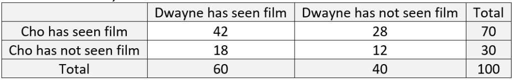
These probabilities are Pr(B) = 59/100 = 0.59 and Pr(B|A) = 42/48 = 0.875.  Learning that Allan has seen the film increases the probability that Beth has seen it considerably.  On the other hand, learning that Cho has seen the film does not change the probability that Dwayne has seen it: Pr(D) = 60/100 = 0.60 and Pr(D|C) = 42/70 =0.60.

  • e) In which case (Allan-Beth) or (Cho-Dwayne) would it make sense to say that the events are independent?

This question is my attempt to lead students to define the term independent events for themselves, without simply copying what I say or reading what the textbook says.  Dwayne’s having seen the film is independent of Cho’s having seen it, because the probability that Dwayne has seen the film does not change upon learning that Cho has seen it.  But Beth’s having seen the film is not independent of Allan’s having seen it, because her probability changes in light of that partial information about the film.

  • f) Based on these data, would you still say that (Allan having seen the film) and (Beth having seen the film) are dependent events, even if they never saw any films together and perhaps did not even know each other?

This question points to a fairly challenging idea for students to grasp.  Probabilistic dependence does not require a literal or physical connection between the events.  In this case, even if Allan and Beth did not know each other, being a similar age or having similar tastes could explain the substantial overlap in which films they have seen.  Similarly, Cho and Dwayne might have watched some films together, but the data reveal that their movie-watching habits are probabilistically independent.


My next example gives students more practice with identifying independent and dependent events, in the most generic context imaginable: rolling a pair of fair, six-sided dice.  Let’s assume that one die is green and the other red, so we can tell them apart. 

Consider these four events: A = {green die lands on 6}, B = {red die lands on 5}, C = {sum equals 11}, D = {sum equals 7}.  For each pair of events, determine whether or not the events are independent.  Justify your answers with appropriate probability calculations.

Here is the sample space of 36 equally likely outcomes:

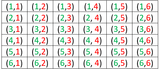
We know that A and B are independent events, because we assume that rolling two fair dice means to roll them independently, so the outcome for one die has no effect on the outcome for the other.  The calculations are Pr(A) = 1/6, Pr(B) = 1/6, Pr(A|B) = 6/36 = 1/6, and Pr(B|A) = 6/36 = 1/6.

It makes sense that A and C are not independent, because learning that the green die lands on 6 increases the chance that the sum equals 11.  The calculations are: P(C) = 2/36 = 1/18 and Pr(C|A) = 6/36 = 1/6.  From the other perspective, Pr(A) = 1/6 and Pr(A|C) = 1/2, because learning that the sum is 11 leaves a 50-50 chance for whether the green die landed on 6 or 5.  The events B and C are also dependent, for the same reason and with the same probabilities.

Some students are surprised to work out the probabilities and find that A and D are independent.  We can calculate Pr(D) = 6/36 = 1/6 and Pr(D|A) = 1/6.  This conditional probability comes from restricting our attention to the last row of the sample space, where the green die lands on 6.  Even though the outcome of the green die is certainly relevant to what the sum turns out to be, the sum has a 1/6 chance of equaling 7 no matter what number the green die lands on.  Similarly, B and D are also independent.

The events C and D also make an interesting case.  Some students find the correct answer to be obvious, while others struggle to understand the correct answer after it’s explained to them.  I like to offer this hint: If you learn that the sum equals 7, how likely is it that the sum equals 11?  I want them to say that the sum certainly does not equal 11 if the sum equals 7.  Then I follow up with: So, does learning that the sum equals 7 change the probability that the sum equals 11?  Yes, the probability that the sum equals 11 becomes zero!*  These events C and D are definitely not independent, because Pr(D) = 2/36 but Pr(D|C) = 0, which is quite different from 2/36.

* Be careful not to read this as zero-factorial**.

** I never get tired of this joke.


Next I show students that if E and F are independent events, then Pr(E and F) = Pr(E) × Pr(F).  Then I provide an example in which we assume that events are independent and calculate additional probabilities based on that assumption.

Suppose that you have applied to two internship programs E and F.  Based on your research about how competitive the programs are and how strong your application is, you believe that you have a 60% chance of being accepted for program E and an 80% chance of being accepted for program F.  Assume that your acceptance into one program is independent of your acceptance into the other program.

  • a) What is the probability that you will be accepted by both programs?
  • b) What is the probability that you will be accepted by at least one of the two programs?  Show two different ways to calculate this.

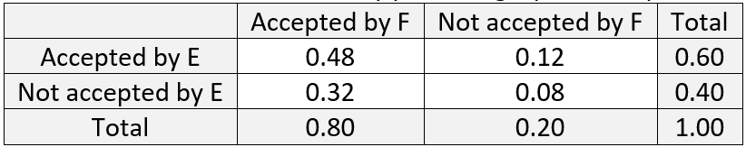
Part (a) is as simple as they come: Pr(E and F) = Pr(E) × Pr(F) = 0.6 × 0.8 = 0.48*.  For part (b), we could use the addition rule: Pr(E or F) = Pr(E) + Pr(F) – Pr(E and F) = 0.6 + 0.8 – 0.48 = 0.92.  We could also use the complement rule and the multiplication rule for independent events, because complements of independent events are also independent: Pr(E or F) = 1 – Pr(not E and not F) = 1 – Pr(not E) × Pr(not F) = 1 – 0.4 × 0.2 = 0.92.  I like to specify that students should solve this in two different ways.  I go on to encourage them to develop a habit of looking for multiple ways to solve probability problems in general. Students could also solve this by producing a probability table:

* You probably noticed that I was a bit lax with notation here.  I am using E to denote the event that you are accepted into program E.  Depending on the student audience, I might or might not emphasize this point.

Next I mention that the multiplication rule generalizes to any number of independent events.  Then I ask: Now suppose that you also apply to programs G and H, for which you believe your probabilities of acceptance are 0.7 and 0.2, respectively.  Continue to assume that all acceptance decisions are independent of all others.

  • c) What is the probability that you will be accepted by all four programs?  Is this pretty unlikely?
  • d) What is the probability that you will be accepted by at least one of the four programs?  Is this very likely?

Again part (c) is quite straightforward: Pr(E and F and G and H) = Pr(E) × Pr(F) × Pr(G) × Pr(H) = 0.6 × 0.8 × 0.7 × 0.2 = 0.0672.  This is pretty unlikely, less than a 7% chance, largely because of applying to very competitive program H.  Part (d) provides much better news: Pr(E or F or G or H) = 1 – Pr(not E and not F and not G and not H) = 1 – Pr(not E) × Pr(not F) × Pr(not G) × Pr(not H) = 1 – 0.4 × 0.2 × 0.3 × 0.8 = 0.9808.  You have a very good chance, better than 98%, of being accepted into at least one program.

  • e) Explain why the assumption of independence is probably not reasonable in this situation.

Even though the people who administer these scholarship programs would not be comparing notes on applicants or colluding in any way, learning that you were accepted into one program probably increases the probability that you’ll be accepted by another, because they probably have similar criteria and standards.  It’s plausible to believe that learning that you were accepted by one school makes it more likely that you’ll be accepted by the other, as compared to your uncertainty before learning about your acceptance to the first school.  This means that the calculations we’ve done should not be taken too seriously, because they relied completely on the assumption of independence.


Next I ask students to consider a context in which independence is much more reasonable to assume and justify:

Suppose that every day you play a lottery game in which a three-digit number is randomly selected.  Your probability of winning for each day is 1/1000.

  • a) Is it reasonable to assume that whether you win or lose is independent from day to day?  Explain.
  • b) Determine the probability that you win at least once in a 7-day week.  Report your answer with five decimal places.  Also explain why this probability is not exactly equal to 7/1000.
  • c) Determine the probability that you win at least once in a 365-day year.
  • d) Suppose that your friend says that because there are only 1000 three-digit numbers, you’re guaranteed to win once if you play for 1000 days.  How would you respond?
  • e) Express the probability of winning at least once as a function of the number of days that you play.  Also produce a graph of this function, from 1 to 3652 days (about 10 years).  Describe the function’s behavior.
  • f) For how many days would you have to play in order to have at least a 90% chance of winning at least once?  How many years is this?
  • g) Suppose that the lottery game costs $1 to play and pays $500 when you win.  If you were to play for that many days (your answer to the previous part), is it likely that you would end up with more or less money than you started with?

Because the three-digit lottery number is selected at random each day, whether or not you win on any given day does not affect the probability of winning on any other day, so your results are independent from day to day.

We will use the complement rule and the multiplication rule for independent events throughout this example: Pr(win at least once) = 1 – Pr(lose every day) = 1 – (0.999)n, where n represents the number of days.  For a 7-day week in part (b), this produces Pr(win at least once) = 1 – (0.999)7 ≈ 0.00698.  Notice that this is very slightly less than 7/1000, which is what we would get if we added 0.001 to itself for the seven days.  Adding these probabilities does not (quite) work because the events are not mutually exclusive, because it’s possible that you could win on more than one day.  But it’s extremely unlikely that you would win on more than one day, so this probability is quite close to 0.007.  I specifically asked students to report five decimal places in their answer just to see that the probability is not exactly 0.007*.

* I like to refer to this as a James Bond probability.

For the 365-day year in part (c), we find: Pr(win at least once) = 1 – (0.999)365 ≈ 0.306.  The friend’s argument in part (d) about being guaranteed to win if you play for 1000 days is not legitimate, because it’s certainly possible that you would lose on all 1000 days.  In fact, that unhappy prospect is not terribly unlikely: Pr(win at least once) = 1 – (0.999)1000 ≈ 0.632 is greater than one-half but much closer to one-half than to one!*

* Feel free to read this as one-factorial.

Here’s the graph requested in part (e) for the function Pr(win at least once) = 1 – (0.999)n:

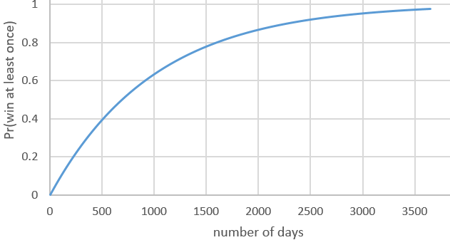
This function is increasing, of course, because your probability of winning at least once increases as the number of days increases.  But the graph is concave down, meaning that the rate of increase gradually decreases as time goes on.  The probability of winning at least once reaches 0.974 after 10 years of playing every day.

Part (f) asks us to solve the inequality 1 – (0.999)n ≥ 0.9.  We can see from the graph that the number of days n needs to be between 2000 and 2500.  Examining the spreadsheet in which I performed the calculations and produced the graph reveals that we need n ≥ 2302 days in order to have at least a 90% chance of winning at least once.  This is equivalent to 2302/365.25 ≈ 6.3 years.  If you’d like your students to work with logarithms, you could ask them to solve the inequality analytically.  Taking the log of both sides of (0.999)n ≤ 0.1 and solving, remembering to flip the inequality when diving by a negative number, gives: n ≥ log(0.1) / log(0.999) ≈ 2301.434 days.

I included part (g) just to make sure that students realize that winning at least once does not mean coming out ahead of where you started financially.  At this point of the course, we have not yet studied random variables and expected values, but I give students a preview of coming attractions by showing this graph of the expected value of your net winnings as a function of the number of days that you play*:

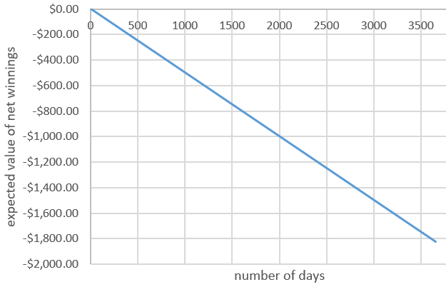
* The expected value of net winnings for one day is (-1)(0.999) + (500)(.001) = -0.499, so the expected value of net winnings after n days is -0.499 × n.


I still have not gotten to my favorite example for independence day, but this post is already long enough.  That example will have to wait for part 2 of this post, which will not be independent of this first part in any sense of the word.

#94 Non-random words

I am teaching a course called Statistical Communication during this spring quarter*.  This course aspires to help Statistics majors, most of whom are completing their second year, to improve their written communication skills with regard to statistical ideas and analyses.  These students have taken at least two statistics courses, and most have taken several more than that.  This class meets synchronously but remotely, with a total of fifty students across two sections.  I am teaching this course for the first time and have never taught a similar course.

* Cal Poly is on the quarter system, so we teach three ten-week (plus finals week) terms per year, not including summer.  Now that we have reached the second half of April, we are three weeks into the Spring term.  We only have one week between quarters, during which we must finish grading for Winter term and then get ready for the Spring term.  Because that’s not much time to prepare for a new course that is very different from any I’ve taught before, I warned my students on day one that I’ll be winging it, figuring out what happens in each class session as we go along.

This post describes a recent class session for this course.  As always, questions that I posed to students appear in italics.


The handout that I prepared for the class meeting bore the same title as this post: Non-random words.  I introduced students to the topic as follows:

One of the challenges in communicating well about statistics and data is that many terms that describe statistical concepts also have meanings in common, everyday conversation.  For some terms, the statistical and everyday meanings match up very well, so the common use can help with understanding the statistical meaning.  But for other terms, the everyday meaning is different enough to provide a hindrance to understanding the statistical meaning.

a) Join a breakout room, and prepare a list of statistical terms that also have common, everyday meanings.  Also think about the statistical and everyday meanings.  Then try to classify each term with regard to how closely the everyday meaning matches the statistical meaning.

I gave students about 12 minutes for this discussion, with 4-5 students in each breakout room.  Before I opened the breakout rooms, I provided an example by pointing to the title of the handout.  I suggested that random is a prime example of a word for which its meanings in everyday conversation are not completely aligned with statistical uses of the word. 

b) We will reconvene as a full class to compile this list and discuss how closely the meanings align.

Some words that my students suggested include: normal, uniform, mean, range, distribution, correlation, significant, confident, independent, risk, odds, chance, effect, control, interaction, block, confounding, sample, population, parameter, factor, response, model, residual, error.

Before class, I had generated my own list.  After giving my students about ten minutes to suggest their words, I looked at my list and found several that had not been mentioned yet: bias, expected, variance, association, statistic, tendency, likelihood, skew.

Next I asked students which words are the most problematic, in that the everyday usage hinders understanding of the statistical meaning.  Some words that students put in this category include: normal, odds, independent, significant, power, control, block.


Our discussion of questions (a) and (b) took more than half of the 50-minute class session.  For the rest of the time, I turned our discussion to an in-depth discussion of the word random:

c) On a scale of 0 – 10, how important would you say the word “random” is in statistics?

I asked students to respond to this question in the zoom chat window*.  All of their responses were on the high side, ranging from 7 to 10, with a majority at 9 or 10.

* I wish that I had thought ahead to prepare this as a zoom poll question.  I think almost all students would have responded to a poll question, whereas only about ten students in each section responded in the chat.

d) What do you think “random” means in everyday (or even slang) usage?

Some common responses were to say surprising, unusual, and unlikely.  Other synonyms offered were odd and weird.  Slightly longer responses included out-of-the-ordinary and out-of-context.  For example, if someone says that a “random” thing happened to them today, they probably mean that it was an unusual, out-of-the-ordinary, occurrence.

A second type of response referred to being haphazard or unpredictable, lacking a pattern or plan.

e) Look up some definitions of “random” in an online dictionary.

I wanted my students to think first for themselves about everyday meanings of “random.”  But then I figured that I should take advantage of knowing that the students are all online during class.  Some dictionary definitions that they provided include:

  • Unknown, unspecified
  • Without method or conscious decision
  • Lacking definite purpose or plan

f) In what ways is “random” used in statistics?

I intended to spend a good bit of time on this question.  Because most students take this course about halfway through their undergraduate career, it provides a good opportunity to review some of the most important topics that they should have learned.  Prior to the class meeting, I had four aspects of “random” in mind for this discussion:

  • Random sampling aims to select a representative sample from a population, so findings about the sample can be generalized to the population.
  • Random assignment tends to produce similar treatment groups, to enable cause-and-effect conclusions if the treatment groups reveal a significant difference in the response.
  • Random selection applies to situations such as choosing a representative from a group of people or dealing out cards in a game.
  • Random variables can model various real-world phenomena, such as waiting time at a fast-food restaurant or number of transactions at an automatic teller machine.

I don’t think I’m very good at leading class discussions, in part because I often have a specific endpoint in mind as I did with this question.  Sometimes I even confess to my students that I’d like them to read my mind, even though I know that’s completely unfair to ask.  In this case my students read my mind quite well and suggested a variation on each of these four aspects of the word “random.”

g) Would you say that the everyday usage of “random” is a help or a hindrance when trying to communicate statistical uses of the word?

Once again, I wish that I had prepared this as a poll question in advance.  Instead I asked students to reply in the chat window, and most of them were reluctant to do that.  Those who volunteered an answer voted for hindrance, which is the response I was hoping for. 

I proposed to students that there is substantial irony here.  In everyday usage random means having no method or plan.  But random sampling and random assignment are very specific methods that require a lot of planning to implement.  Similarly, a random variable provides a very specific, predictable pattern for the long-run behavior of what it’s modeling, even though the outcome of a specific instance is unpredictable.


I try to think a lot about what kind of assessments to provide after a class session like this.  In this case, I made two small assignments and am contemplating a third, more substantial one.

I’ve mentioned many times that I give lots of quizzes in my courses.  Following this class session, I gave my students a very easy quiz.  I simply asked them to select their five favorite words that illustrate the distinction between everyday and statistical meanings.  I realize that this quiz amounted to giving free points for showing up to class, paying a modest amount of attention, and taking a few minutes to respond in Canvas.  But I hope students gave a little reflection as they answered, and I enjoyed reading their responses to see which words most resonated with them.

I also created a discussion in Canvas in which I asked students: Describe an example that uses a word with a specific statistical meaning in a way that carries a different meaning than the statistical one.  I’m thinking of the words that we discussed and listed in connection with the “Non-random Words” handout. Be very clear about which word(s) you are referring to.  Also describe what you perceive to be the intended meaning of the word(s).  If you found the example online, include a link.  I kicked off this discussion with an example that had appeared in my inbox just that morning: I received an email message inviting me to attend a webinar titled “A Conversation on Power, Structural Racism, and Perceptions of Normality in STEM Through a Lens of Critical Race Theory.”  The statistical words used in non-statistical ways are power and normality.  In this context, power refers to authority or control over others, and normality refers to what is typical or expected.  Here is a link to the webinar announcement.

I am also considering asking students to write an essay with these instructions: Select one of the words that we identified in class.  Write an essay of 250-400 words in which you describe how the statistical meaning of the word compares to the everyday meaning.  Mention similarities as well as differences, if there are similarities.  Provide at least one example to explain the word’s meaning in statistics.  Write as if to a relative of yours who is well-educated and intellectually curious but has not specialized in a STEM field and has never taken a statistics course.  Be sure to cite any references that you use (e.g., dictionary, textbook, wikipedia, …)

I have not given this assignment yet, because I am trying to balance students’ workload (and my grading load) with other assignments.  I am also debating whether I should ask them to select from a small list of words that I provide, such as: normal, bias, error, power, independent, expectation.


I realize that few readers of this blog are teaching a course called Statistical Communication.  I suspect that you might be thinking: What does this have to do with teaching introductory statistics*? 

* Even though I italicized this question for emphasis, this one is directed at myself and perhaps you, rather than students.

Many words have slightly or substantially different meanings in statistics than in everyday conversation, which can present a hurdle for introductory students to overcome.  I think we can help students by highlighting such discrepancies, as with the word random.  By pointing out that such words have a particular meaning in statistics that differs from what students might expect*, we can help them to concentrate on the statistical meanings that we’d like them to learn.  Also, even though few courses have the word “communication” in their title, many introductory courses have an explicit or implicit learning objective to help students learn to communicate effectively with data.

* By all means, do not expect the statistical meaning of the word expect to mean what your students might expect.  See post #18, titled What do you expect?, here.

#93 Twenty-one questions about USCOTS ’21

Registration for the 2021 U.S. Conference on Teaching Statistics (USCOTS) opens today.  I’m so excited about this that I will devote this blog post to answering 21 questions that you may have* about this conference**.

* You may not even have realized that you have these questions until you read them.

** I also wrote a bit about USCOTS in a meandering and autobiographical post #76, titled Strolling into serendipity, here.


1. Where can I register?  Follow the link here.

2. How much is the registration fee?  $25.  If this would constitute a hardship, you can receive a full waiver.

3. When is it?  The conference runs from June 28 – July 1.  Sessions will run from approximately 11:30am – 5:30pm Eastern time (U.S.) on each day.  Pre-conference workshops begin on June 24.

4. Where is it?  USCOTS will be held virtually for the first time this year, so it’s happening wherever you and your internet connection happen to be at the time.

5. Why should I attend USCOTS?  (Thanks for asking.  I really should have started there, shouldn’t I?)  Many statistics conferences include sessions on teaching, and many teaching conferences include sessions on statistics, but USCOTS is devoted entirely to the challenge of teaching statistics well.  If you teach statistics at the undergraduate or high school level, you will find sessions that are relevant to your everyday work in every time slot.  Our goal is for every session to include both practical advice and thought-provoking ideas, and also to present them in an engaging, perhaps even fun, manner.  If you’ve never attended USCOTS, we welcome you and hope that you’ll meet some new friends.  If you have attended USCOTS, we welcome you back to renew acquaintances.  We hope that you’ll be inspired to improve your teaching of statistics.

6. What is the conference theme?  Expanding opportunities.

7. Can you say more about that?  We encourage presenters and attendees to interpret this theme broadly, but we primarily have two questions in mind:

  • How can we (teachers of statistics and others involved with statistics education) increase participation and achievement in studying statistics by students from underrepresented groups?
  • How can we better encourage and support students and colleagues who are beginning or contemplating careers in statistics education?

8. What kind of sessions are planned?  Each of the four days will feature a keynote presentation and interactive breakout sessions.  We’ll also have “posters and beyond” presentations, “birds-of-a-feather” discussions, and exhibitor demonstration sessions.  New this year will be a speed mentoring session.  Another highlight will be an awards presentation ceremony.  Speaking of highlights, I almost forgot to mention my own favorite: Opening and closing sessions will feature lively five-minute presentations on the conference theme.  You can see the conference program here.

9. Who are some of the presenters?  The keynote speaker for Monday is Rebecca Nugent from Carnegie Mellon.  She will discuss how the emerging field of data science can expand opportunities for students who have been under-represented in statistics.  Tuesday’s keynote presentation will be a panel discussion about expanding horizons and fostering diversity, with panelists Felicia Simpson, Jacqueline Hughes-Oliver, Jamylle Carter, Prince Afriyie, and Samuel Echevarria-Cruz.  On Wednesday Catherine D’Ignazio and Lauren Klein will discuss theme from their book Data Feminism.  Alana Unfried from California State University – Monterey Bay will give Thursday’s keynote presentation.  She will discuss the advantages of a co-requisite model that enables students needing remediation to enter directly into an introductory statistics course.

10. What are some of the workshop topics?  These topics include community-engaged learning, data visualization, data science, Bayesian statistics, R tidyverse, games, multivariable thinking, and statistical literacy.  You can see the list of pre-conference workshops here.

11. How about some of the breakout session topics?  These topics include data science, social justice, gamification, communication skills, oral assessments, computational thinking, data visualization, community building, educational fun, and data ethics.  You can find the list of breakout sessions here.

12. What platforms will the conference use?  The primary platform will be zoom.  You can attend sessions simply by following zoom links.  We’ll make frequent use of breakout rooms, polls, and chat within zoom to increase engagement.  We will also use gather.town to replicate an in-person experience more closely.

13. Will the conference be interactive and engaging?  That’s our goal.  I think this is more challenging with a virtual conference than with an in-person one, but we’ll do our best.  Of course, interactivity and engagement depend on participants being willing* to interact and engage.

* I hope eager!

14. Can I still submit a proposal to present at the conference?  Yes.  Proposals for “posters and beyond” sessions are due by April 22 (here).  Proposals to lead a birds-of-a-feather discussion are due by May 31 (here).

15. How can I earn a free registration?  Participate in the SPARKS video challenge.  This asks for a very short (10-20 seconds) video clip that can be used in teaching statistics.  You can see examples and submit your entry here.

16. Do you have a social media hashtag in mind?  Yes, please use #USCOTS21.

17. Would you like me to spread the word to colleagues and friends?  Yes, absolutely!

18. Do I have to attend every minute of every session of the conference?  No.  (Whew, I’m glad to have a chance to introduce some variability to that long string of “yes” answers that I have been giving.)  Feel free to tune in when you can and step away when you need to.  As you would expect, I think it would be ideal if you can block out several hours of uninterrupted time for each day of the conference, but of course I realize that your circumstances may not allow that.

19. Can I see what has happened in previous USCOTS conferences?  I can resume my “yes” answers again.  See the links for “previous years” on the right side of the main conference page here.

20. Do you happen to have a one-minute video with a musical invitation to attend USCOTS that I could watch and point others to?  Yes*!  Thanks to the creativity and talents of Larry Lesser and Mary McLellan, please enjoy the video here.

* Wow, what a great question; it’s like you were reading my mind!

21. Please remind me: how can I register?  Just follow the link here.

#92 What can you do?

Teachers are often asked: What can you do with …?  For example, many students and prospective students have asked me: What can you do with a degree in statistics? 

I used to find it very challenging to answer this question well.  One reason is that I have never had a job other than college professor.  Don’t get me wrong: I love my job, and I would make the same choice again, without a second thought, if I were starting over.  But my career has not provided me with much first-hand experience for answering that question.

I eventually came up with an answer that I really liked.  I came to give this answer every time I heard the question.  I still give the same answer now.  In fact, I like this answer so much that I put it on the back of my business cards. 

My answer is: https://statistics.calpoly.edu/news/2021-alumni-notes-2019-2020.  There you can find  the alumni updates section of our department newsletter*.  I am referring to the Department of Statistics at Cal Poly – San Luis Obispo.  We have had a bachelor’s degree program in statistics since the mid-1970s, and we are very proud of our alums.

* You can also find previous editions of the newsletter here and here.


Why do I like this answer so much?  Let me count the ways:

  1. This answer relies on other people’s words, not mine.  Because I do not have much relevant first-hand experience for addressing this question, I am very happy to refer to others’ experiences.
  2. These people have an undergraduate degree in statistics and are out in the “real world.” Most are outside of academia, applying what they’ve learned.
  3. Our alums have experienced diverse work experiences.  Many work very closely with data and statistics on a daily basis, but others’ careers are only tangentially related to data, if at all.  Some are not using their academic background in statistics at all, which I think is valuable for demonstrating that what you study as an undergraduate does not dictate what you have to do with the rest of your life.
  4. Needless to say, these are real people with real lives, including families and hobbies and interests that are not related to statistics at all.  I think it’s nice for current and prospective students to see that these folks have families, weddings (some to fellow alums of our program), children, pets, hobbies, (pre-pandemic) travel adventures, and more.
  5. This answer fits on the back of a business card.

Communicating with our alums to solicit these updates was one of my favorite tasks when I recently served as department chair for six years.  In fact, I enjoyed this activity so much that I volunteered to continue after I completed my terms from my chair.  I am very proud that so many of our alums take the time to respond with an update; 73 responded for the most recent edition, and even more replied for the two previous editions.

A big part of my enjoyment is that I taught many of these students, so of course it’s fun for me to hear from them and learn about what they’re up to, both professionally and personally.  I realize that you do not know these Cal Poly alums personally*, but I’m hoping that you might enjoy reading about the kinds of careers that people with undergraduate degrees in statistics can pursue.  I will provide a brief summary in this post, but I highly recommend that you follow the links above to read their words directly for yourself**.

* Unless you are one of my Cal Poly colleagues, or perhaps even one of the Cal Poly alums who contributed an update

** You’ll find that the updates are spread across many pages, arranged by graduating class year.  Click on links at the bottom of the pages to see more updates.


Many of the job titles for these alums include the terms data scientist or data analyst.  Some other terms include data quality analyst, research analyst, risk consultant, actuary, software engineer, SAS programmer, or R programmer.

The industries in which these alumni work run the gamut, including banking, insurance, financial services, health care, fashion, marketing, medicine, pharmaceuticals, biotechnology, social media, gaming, entertainment, education, and more.

Some alums are pursuing or have completed graduate degrees, in fields such as statistics, biostatistics, public health, data science, business analytics, computer science, computational science, psychology, and education.

A few of the alums almost apologize for not using statistical methods in their daily work.  But they generally say that learning how to think about data and solve problems has served them well.  For example, Alex wrote that our year-long sequence in mathematical statistics “taught me to think ‘why’ instead of just ‘how.’”  Cisco contributed that “the most important thing that I learned from statistics and still use is the thought process to take big generic problems and turn them into manageable steps toward improvement.”


That summary was brief, as promised, but very dry.  Like I said, I’d prefer that you read the alums’ words rather than mine (again, here and here and here). Rather than delete my dry summary, let me instead try to add some life by highlighting a few specific updates. I hope these might help to persuade you to read them all :

  1. Maddie works as a financial data analyst for a solar energy company during the week.  On weekends she works at a residential care facility for adolescent girls with anxiety disorders.
  2. Jianyi started by working for a non-profit organization while launching her own cake-baking business.  Now she works as a production manager and data analyst for a company that designs lighting accessories.
  3. Alicia taught at an all-girls Catholic high school in Sacramento and now teaches statistics and calculus at Sacramento State University.  She also writes and performs comedy sketches, is writing a screenplay, and writes a blog here.
  4. Upneet moved to a city in which probability plays a large role in the economy: Las Vegas.  She works as an analyst at the Venetian/Palazzo Hotel and Casino in Las Vegas.
  5. Caiti has held positions as a data scientist for two companies that I suspect you have heard of: The Gap, Inc. and Google.
  6. David started his career as an engineer for Disney.  Now he is co-founder of an e-sports social media start-up company.
  7. Hunter earned his Ph.D. in Statistics and returned to Cal Poly as a faculty member in our department.  He has recently earned tenure, and he has also co-authored a blog on teaching data science (here).
  8. Chris heads up the data effort for a video game start-up company in Berlin.  He has helped the video game industry to become more data-driven, implementing more sophisticated methods and technologies.
  9. Emily taught AP Statistics for a decade before becoming Mathematics Coordinator for the Merced County Office of Education.  One of her initiatives involves developing a data science course to offer high school students an additional mathematics pathway to college readiness*.
  10. Kendall also taught AP Statistics for a decade, until he recently bought a coffee farm on the Big Island of Hawaii, where he also works on a dive boat.

* This is far from her most impressive accomplishment, but Emily wrote a guest post for this blog (here).


What can you do with a degree in statistics?  The American Statistical Association has some great materials for answering this question, including their This is Statistics project (see here and here).

For students attending or considering Cal Poly, I like my answer of pointing them to alumni updates (once again, for the final time, see here and here and here).  I hope that this answer might also be a reasonable one for you to offer to your students.  Even better, you could reach out to your own former students and compile their updates.

I have greatly enjoyed using our department newsletter as a vehicle for keeping in touch with alums.  I focus a lot of my teaching effort on preparing handouts and activities, developing and grading assessments*.  These alumni updates provide me with a reminder that the most important part of teaching is helping students to learn and prepare for their careers and lives.

* Remember: Ask good questions.

Because this post has extolled the virtues of reading words other than my own, I will conclude with advice and encouragement from Jose, who graduated from Cal Poly with a degree in Statistics in 1993: Think about what’s fulfilling for the soul and not the bank account….  These are exciting times for statisticians and anyone analytically inclined. Predicting the future with confidence and with limited data was never more important and exciting.