My break from writing this blog continues. I look forward to resuming soon.
In the meantime, I thank all who attended USCOTS (U.S. Conference on Teaching Statistics) earlier this summer. If you were not able to attend, or if you missed some of the keynote sessions, or if attended and would like to re-watch them, please see the recordings that Bob Carey has prepared and posted. You can find these recordings by scrolling down on the session pages linked below:
Opening session of five-minute talks on the conference theme of “Expanding Opportunities,” featuring Anna Fergusson, Frank Savina, Jennifer Green, Kathryn Kozak, Maria Tackett, and Rebecca Wong (here)
Democratizing Data (Science): Empowering and Expanding Opportunities for Both Students and Educators, by Rebecca Nugent (here)
Panel discussion on “Expanding Horizons and Fostering Diversity,” featuring Felicia Simpson, Jacqueline Hughes-Oliver, Jamylle Carter, Prince Afriyie, and Samuel Echevarria-Cruz (here)
Data Feminism, by Lauren Klein and Catherine D’Ignazio (here)
Data Science Ethics: A Checklist for Statistics Educators, by Jessica Utts (here)
Expanding Opportunities for Underprepared Statistics Students, by Alana Unfried (here)
Closing session of take-away thoughts on “Expanding Opportunities,” featuring program committee members Amy Hogan, Camille Fairbourn, Eric Reyes, Judith Canner, Kelly Spoon, Larry Lesser, Megan Mocko, Sharon Lane-Getaz, and Todd Iversen (here)
The U.S. Conference on Teaching Statistics (USCOTS) begins today! Please join us to consider the conference theme of “Expanding Opportunities” by following links from the conference program website here.
I interrupt my break from blogging to remind you that the 2021 U.S. Conference on Teaching Statistics (USCOTS) begins in just one week! I am eagerly looking forward to this virtual conference, which will feature many session on the theme of “Expanding Opportunities.” I hope that you’ll join me, my co-program chair Kelly McConville, and hundreds of other teachers of statistics at USCOTS from Mon June 28 – Thur July 1.
As I mentioned at the end of last week’s post (here), I am taking a break for a month or two. If you have missed any of the first 100 posts in the Ask Good Questions blog, please check them out over the summer.
Thanks very much for reading! Please check back in August. And please consider attending USCOTS (here) at the end of June.
In posts #95 and #99 (here and here), I described examples that my students work through when we study the probability concept of independent events. Now in part 3 of this series, I will describe three assessment items that I have used for this topic. The first is a single question. The second is a five-question, auto-graded quiz. The third is a multi-part assignment. In addition to giving students practice working with probabilities involving independent events, each of these assessments also aims to sneak in another topic from probability or statistics.
As always, questions that I pose to students appear in italics.
1. Suppose that a researcher conducts 20 independent tests, each of which has a 5% chance of resulting in an error. Determine the probability that at least one of these tests results in an error.
This question is similar to the example (from post #95, here) involving a daily lottery number. The solution is: Pr(at least one error) = 1 – Pr(no errors) = 1 – Pr(first test does not result in an error and second test does not result in an error and … and twentieth test does not result in an error) = 1 – (1 – 0.05)^20 = 1 – (0.95)^20 ≈ 0.642.
When I discuss this question in class, I point out that this calculation reveals a problem with conducting a large number of tests. Even with a small probability of error on any one test, performing a large number of tests results in a substantial probability of committing at least one error. This is a primary objection to the ill-advised practice sometimes known as p-hacking. This xkcd cartoon (here) provides a wonderful illustration of p-hacking.
2. Suppose that the two sports teams, the Domestic Shorthairs and the Cache Cows, play a series of games. Assume that the results of the games are independent and that the Domestic Shorthairs have a 0.6 probability of winning each game.
a) What does it mean to say that the results of the games are independent? [Options: A) The probabilities of winning later games do not change, regardless of which team wins earlier games. B) Each team has a 50-50 chance to win each game. C) It’s impossible for the same team to win two games in a row. D) Whichever team wins a game has a larger probability of winning the next game. E) Whichever team wins a game has a smaller probability of winning the next game.] The correct answer is A), but option B) can entice many students.
b) Determine the probability that the Domestic Shorthairs win the first two games of the series. Applications of the multiplication rule for independent events do not come simpler than this. If we let W denote a win and L a loss for the Domestic Shorthairs, this probability is calculated as: Pr(W1 and W2) = Pr(W1) × Pr(W2) = 0.6×0.6 = 0.36.
c) Determine the probability that the Domestic Shorthairs win two games before the Cache Cows win two games. This question is somewhat similar to “unfinished game” example from post #99, here. This probability can be calculated as: Pr[(W1 and W2) or (W1 and L2 and W3) or (L1 and W2 and W3)] = 0.6×0.6 + 0.6×0.4×0.6 + 0.4×0.6×0.6 = 0.648. When I present this as an in-class example rather than an out-of-class assessment, I first ask students to predict, without performing calculations, whether the answer will be equal to 0.6, less than 0.6, or greater than 0.6.
d) Suppose that the Domestic Shorthairs’ probability of winning each game was larger than 0.6. How would this change the probability that the Domestic Shorthairs win two games before the Cache Cows win two games? [Options: A. No change, B) Increase, C) Decrease] This question is meant to be quite easy: A larger probability of winning any one game also leads to a larger probability of winning the series, so the correct option is B).
e) Now suppose that you are a fan of the Domestic Shorthairs and want them to win the series of games against the Cache Cows. Assume again that the Domestic Shorthairs have a 0.6 probability of winning any one game and that game results are independent from game to game. Would you prefer them to play a single game, a best-of-three series, or a best-of-five series? [Options: A) Single game, B) Best-of-three, C) Best-of-five, D) No preference] The correct answer here is C). A longer series favors the stronger team. From the opposite perspective, the underdog would prefer to play a single game rather than a longer series, in which the better team is more likely to demonstrate its superiority. This question sneaks in the idea that a larger sample size is more likely to produce a sample result similar to the truth about the population. If this were not an auto-graded quiz, I would ask students to explain their answer for part (e).
The next question is a fairly long assignment with ten parts. This assignment introduces students to connections in series and connections in parallel. Most of these parts ask typical questions, so you might want to skip ahead to the more interesting parts (i) and especially (j).
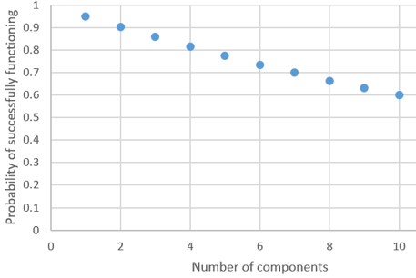
3. Consider a system that requires all components to function successfully in order for the system to function successfully. (Such a system is said to be connected in series.) Suppose that the components operate independently and that the probability that a single component functions successfully is 0.95.
a) Determine the probability that a system with two components connected in series functions successfully. Also indicate the probability rule(s) that you use for this calculation.
b) Now suppose that the system consists of three components connected in series. Determine the probability that this system functions successfully. Is this probability larger, smaller, or the same as with two components?
c) Now suppose that the system consists of n components (where n is a positive integer) connected in series. Determine the probability that this system functions successfully, as a function of n.
d) Produce a graph of this function from c), for integer values of n from 1 to 10. (Label both axes clearly.) Also describe the behavior of this function.
If we let Si represent the event that component i functions successfully, the probability in part (a) is: Pr(S1 and S2) = Pr(S1) × Pr(S2) = (0.95)^2 = 0.9025, using the multiplication rule for independent events. Similarly, Pr(S1 and S2 and S3) = (0.95)^3 ≈ 0.857, which is a smaller probability. The general expression is: Pr(S1 and S2 and … and Sn) = (0.95)^n. This function decreases gradually, as shown in the graph below. This decrease makes sense because, as a single bad component is all that’s needed to cause the system to fail, each additional component provides another opportunity for such failure.
Now consider a system of components that requires at least one component to function successfully in order for the system to function successfully. (Such a system is said to be connected in parallel.) Continue to suppose that the components operate independently, but now suppose that the probability that a single component functions successfully is 0.25.
e) Determine the probability that a system with two components connected in parallel functions successfully. Also indicate the probability rule(s) that you use for this calculation.
f) Now suppose that the system consists of three components connected in parallel. Determine the probability that this system functions successfully. Is this probability larger, smaller, or the same as with two components?
g) Now suppose that the system consists of n components (where n is a positive integer) connected in parallel. Determine the probability that this system functions successfully, as a function of n.
h) Produce a graph of this function from g), for integer values of n from 1 to 10. (Label both axes clearly.) Also describe the behavior of this function.
The probability calculations here are: Pr(S1 or S2) = Pr(S1) + Pr(S2) – Pr(S1 and S2) = 0.25 + 0.25 – (0.25)^2 = 0.4375 by the addition rule and the multiplication rule for independent events. An alternative solution that uses the complement rule is: Pr(S1 or S2) = 1 – Pr[(not S1) and (not S2)] = 1 – (0.75)^2 = 0.4375. With three components, this becomes: Pr(S1 or S2 or S3) = 1 – Pr[(not S1) and (not S2) and (not S3)] = 1 – (0.75)^3 ≈ 0.578. This probability is larger than with three components. The general expression is: Pr(S1 or S2 or … or Sn) = 1 – Pr[(not S1) and (not S2) and … and (not Sn)] = 1 – (0.75)^n. This function increases somewhat rapidly, as shown in the graph below. This makes sense because, as only one successful component is needed, each additional component now provides another opportunity for the system to succeed.
Now suppose that a system consists of three components. Two of the components are connected in parallel to form a sub-system. That sub-system is then connected in series with the third component. Continue to suppose that the components operate independently. Now suppose that the probability is 0.9 that a single component functions successfully.
i) Determine the probability that the system functions successfully. Also indicate the probability rule(s) that you use for this calculation.
The system will function successfully if at least one of two components connected in parallel function successfully, and the third component functions successfully. This probability can be calculated as: Pr[(S1 or S2) and S3] = Pr(S1 or S2) × Pr(S3) using the multiplication rule for independent events, which = [Pr(S1) + Pr(S2) – Pr(S1 and S2)] × Pr(S3) using the addition rule, which = (0.9 + 0.9 – 0.81) × 0.9 = 0.99 × 0.9 = 0.891.
Finally, suppose that:
Component A functions successfully with probability 0.8.
Component B functions successfully with probability 0.7.
Component C functions successfully with probability 0.6.
You can select which two components to connect in the parallel sub-system and which component to connect in series to that sub-system.
j) Which component would you select to be connected in series, in order to produce the greatest probability that the system functions successfully? Explain your answer, and also calculate the probability that the system functions successfully with your configuration.
The component connected in series is the one that has to function successfully in order for the system to function successfully. So, the optimal arrangements puts the most reliable component (A) in that series connection and the other two in the parallel connection. The probability is therefore: Pr[(SB or SC) and SA] = Pr(SB or SC) × Pr(SA) = [Pr(SB) + Pr(SC) – Pr(SB and SC)] × Pr(SA) = [0.6 + 0.7 – (0.6)(0.7)] × 0.8 = 0.88 × 0.8 = 0.704.
This last part is my favorite question in the assignment, because it asks students to think before they calculate. I want students to realize that the best component should be placed in the most important position. Students can also calculate probabilities for the other two arrangements to confirm that their intuition is correct. These probabilities turn out to be [0.6 + 0.8 – (0.6)(0.8)] × 0.7 = 0.92 × 0.7 = 0.644 and [0.7 + 0.8 – (0.7)(0.8)] × 0.6 = 0.94 × 0.6 = 0.564, both of which are indeed smaller than 0.704.
This concludes a three-part series on studying independent events*. The first two posts presented examples and activities that I often use in class, and this one has suggested some out-of-class assessment questions.
* I am kicking myself about timing, because I wish that I had planned for this Independence Day series to conclude on the Fourth of July rather than on Memorial Day.
P.S. Speaking of timing, you may have noticed that this is the 100th consecutive weekly post in the Ask Good Questions blog. That’s such a momentous number in our base 10 system that I am going to take the next month or two off. Thanks very much to all who have invested some of your most precious commodity – your time – into reading my blog posts. I look forward to resuming again after this pause, and I hope very much that you will rejoin me then.
P.P.S. I also hope to see you at the U.S. Conference on Teaching Statistics (USCOTS), which will occur virtually on June 28 – July 1, with pre-conference workshops beginning on June 24. We have lined up a terrific program to address the theme of “Expanding Opportunities.” You can peruse the program here, register (for just $25, which can be waived) here, and read my previous blog posts about USCOTS here and here.
In post #95 (here), I described several examples for introducing students to the concept of independent events. This post presents two more examples that I like to use on Independence Day. As always, questions that I pose to students appear in italics.
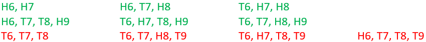
I present my students with the following scenario, which is a simplified version of the famous problem discussed by Pascal and Fermat that led to the development of probability theory, described in the book The Unfinished Game, by mathematician Keith Devlin:
Suppose that Heather and Tom play a game that involves a series of coin flips. They agree that if 5 heads occur before 5 tails, then Heather wins the game. But if 5 tails occur before 5 heads, then Tom wins the game. They each agree to pay $5 to play the game, so the winner will make a profit of $5. The first five coin flips result in: H1, T2, T3, H4, H5. Unfortunately, the game is interrupted at that point and can never be finished.
a) Suggest a reasonable way to divide up the $10. The two most common responses that my students offer are: 1) give each person their $5 back, or 2) give Heather $6 and Tom $4 because Heather has won 60% of the first 5 coin flips. I tell students that these are perfectly reasonable suggestions, but mathematicians proposed to divide the $10 based on the probabilities that each player would have gone on to win the game if it had been continued.
b) Make a guess for the probability that Heather would have won the game if it had been continued. I do not ask students to reveal their guesses, but I want them to give this some thought before proceeding to analysis.
c) List the sample space of ten possible outcomes for how the game could have ended up. Use similar notation to above. This can be tricky for students, so I sometimes give a hint: Six outcomes lead to Heather’s winning, and four outcomes lead to Tom’s winning. For students who still need some help, I ask: What’s the quickest way for the game to end? At this point a student will say that Heather will win if the next two flips produce heads. Then we’re off and running. The sample space is shown below, with outcomes for which Heather wins in green and outcomes for which Tom wins in red:
d) Is it reasonable to regard these 10 outcomes as equally likely? Explain why or why not. This can give students pause, until they realize that some outcomes involve two coin flips, some three, and some four. Because of these differing numbers of flips, it’s not reasonable to regard these outcomes as equally likely.
e) Is it reasonable to regard the coin flips as independent? Explain. Assuming independence is reasonable here, because the result of any one coin flip should not affect the 50-50 chance for any other coin flips’ results.
f) For each player, determine the probability that they would win the game, if it were completed from the point of interruption. Also interpret this probability. Calculating these probabilities involves realizing that:
An outcome of either H or T has probability 0.5 for any one flip.
Independence of coin flips means that these 0.5 probabilities are multiplied to determine the probability for an outcome of multiple flips.
This produces a probability of (0.5)n for all possible outcomes of n coin flips.
So, all two-flip outcomes have probability (0.5)2 = 0.25. All three-flip outcomes have probability (0.5)3 = 0.125. And all four-flip outcomes have probability (0.5)4 = 0.0625.
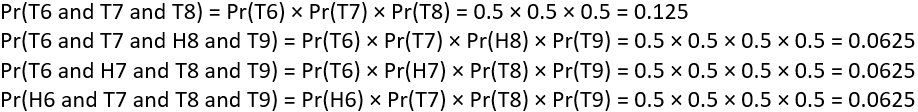
More formally, we can calculate the probabilities for the six outcomes in which Heather wins the game as follows:
For students who get stuck at this stage, I ask: What do we do with these six probabilities to calculate the (overall) probability that Heather would win if the game were completed from the point of interruption? Someone invariably answers that we add them, to which I respond: Yes, but why is that appropriate? This question is slightly harder, but eventually someone will point out that these six events are mutually exclusive. This sum turns out to be 0.6875.
Now I ask: What’s the easy way to calculate the probability that Tom would win the game? A student will point out that we can simply subtract Heather’s probability from one. I agree but suggest that we go ahead and figure out Tom’s probability from scratch. Then we can make sure that the two probabilities sum to one, as a way to check our work. Here are the calculations for outcomes in which Tom wins the game:
Adding these probabilities does indeed give 0.3125 for Tom’s probability of winning.
g) Based on this probability, how should the $10 be divided? If we agree to distribute the $10 proportionally to the probabilities of winning the game if it had been finished from the point of interruption, then Heather should take $6.875 and Tom $3.125. Good luck with that extra half-cent.
h) What is the probability that the game would require four more coin flips to finish? I ask this question to reinforce the idea that we can add the probabilities for the (mutually exclusive) outcomes that comprise this event. Six outcomes require four more flips, and each of those outcomes has probability (0.5)4 = 0.0625, so this probability is 6(0.0625) = 0.375.
The last example that I present on Independence Day is my favorite:
Consider four six-sided dice, all equally likely to land on any one of the six sides, but without the usual numbers 1-6 on the sides. Instead the six sides have the following numbers:
Die A: 4, 4, 4, 4, 0, 0
Die B: 3, 3, 3, 3, 3, 3
Die C: 6, 6, 2, 2, 2, 2
Die D: 5, 5, 5, 1, 1, 1
Suppose that you and I play a game in which we each select a die and roll it independently of the other. The rule is very simple: Whoever rolls the larger number wins. Being a considerate person, I let you select your die first. For whichever pair of dice that you and I might select, determine the probability that I win the game.
I wait for a student to select a die. Let’s say that she selects die B. Think about which die I should select to play against die B. I announce that I will select die A. Notice that I will roll a larger number, and therefore win the game, whenever die A lands on 4. Because four of the six sides of die A have the number 4, the probability that I win is 4/6 = 2/3 ≈ 0.6667.
Now I ask my students to make a different initial selection. Let’s say that someone selects die C. Think about which die I should select to play against die C. This time I will select die B. Notice that I will roll a larger number, and therefore win the game, whenever die C lands on 2. Because four of the six sides of die C have the number 2, the probability that I win is again 4/6 = 2/3 ≈ 0.6667.
At this point, some students begin to catch on, but I persist and ask for a different initial selection. Now suppose that a student selects die D. Think about which die I should select to play against die D. Now I will select die C. Why is the probability calculation more complicated this time? Because we have to two ways for me to win, one of which depends on what number you roll. In other words, we need to consider intersections of events. This time I will win when die C lands on 6, or when die C lands on 2 and die D lands on 1. We could express this as: Pr[C6 or (C2 and D1)]. We can calculate this as: Pr(C6) + Pr(C2)×Pr(D1), where the multiplication is justified because C2 and D1 are independent events. This works out to be (surprise, surprise): (2/6) + (4/6)×(3/6) = 2/3 ≈ 0.6667.
Most students have caught on by now, but I insist on finishing this story. The only other option is for you to select die A, in which case I will select die D. Can you guess the probability that I win this time? No surprise, this probability is now: Pr[D5 or (D1 and A0)] = (3/6) + (3/6)×(2/6) ≈ 0.6667.
What’s the best way to play this game? Convince your opponent to select a die first. No matter which die they choose, you can always select a die that gives you a 2/3 chance of winning the game.
What mathematical property does this example violate? Usually, one student will tentatively suggest the correct answer, that this example violates the transitive property. This property would say that because die A beats die B 2/3 of the time, and die B beats die C 2/3 of the time, and die C beats die D 2/3 of the time, you would expect die A to beat die D at least 2/3 of the time. But the opposite is true, because we have established that die A beats die D only 1/3 of the time. This is sometimes called an example of non-transitive dice.
I find this example amusing, and I think some of my students agree. I enjoy ending our Independence Day class with this flourish.
These two examples do not introduce students to new probability concepts or methods or rules. They simply provide opportunities to apply the multiplication rule for independent events. The unfinished game example gives me a chance to mention the history of probability. The non-transitive dice example is just plain fun.
I also want to describe some quiz and homework questions that I ask as a follow-up to these Independence Day examples, but I’ll save those for part 3 of this series.
I hope that students in my Statistical Communication course make less grammar mistakes after taking my course then they would of beforehand.
Whoops, let me try that again: I hope that students in my Statistical Communication course make lessfewer grammar mistakes after taking my course thenthan they would ofhave beforehand.
I beg you’re your indulgence as I ignore statistics and it’s its teaching in this post, instead turning my attention to grammer grammar. If these opening sentences do not appeal to you, than then theirthey’re there is little chance that you will enjoy this post, so I suggest that you read no farther further. On the other hand, if this paragraph peakspeaks piques your curiosity, then please take a peakpique peek at the rest of this post. I hope that itsit’s worth the time that your you’re investing, with the piquepeek peak of you’re your enjoyment still to come.
I thought about trying to develop an informative and fun in-class grammar activity that my Statistical Communication students could engage in during a live zoom session. But* I decided to make this an asynchronous activity instead. I asked the students to read through the grammatical advice provided here. Then I gave them an online, auto-graded quiz that I hope prompted them to think through some grammar issues. For each quiz question, students filled in blanks to complete sentences correctly, selecting from two or more options presented for each blank. My goals in writing these sentences were to:
keep them brief,
use contexts involving data or statistics,
address many grammatical issues,
use a total of ten sentences, and
amuse myself.
* One of my favorite pieces of writing advice is that once you have learned rules of grammar, you’re welcome to break them when you have a good reason. I have come to like starting an occasional sentence with But.
I know that I succeeded with the last two goals in this list. I think I achieved some success with the second and third goals. My favorite sentences are the last two, because they achieve the first goal with considerable economy of words. In case you’d like to take this quiz for yourself, I will mix up the order of the options, and I present correct answers at the end of this post.
Without fartherfurtheradieuado, hearhereisare the quiz questions:
Select the appropriate words to fill in the blanks to make the sentence grammatically correct:
1. The experimenters will [blank1] five subjects to each treatment, which is not [blank2]. Options for blank1: alot, allot, a lot. Options for blank2: alot, allot, a lot.
2. They should [blank3] found that the treatment group has a smaller infection rate [blank4] the control group. Options for blank3: of, have. Options for blank 4: then, than.
3. My topic generates [blank5] interest than other professor’s topics, so [blank6] students enroll in my course. Options for blank5: less, fewer. Options for blank6: less, fewer.
4. About the outlier, [blank7] important to investigate [blank8] [blank9] on the analysis. Options for blank7: it’s, its. Options for blank8: it’s, its. Options for blank9: affect, effect.
5. You earned a [blank10] from your teacher for including a graph to [blank11] your verbal description. Options for blank10: complement, compliment. Options for blank11: complement, compliment.
6. Your data [blank12] my interest, so let me [blank13] at your histogram to see where the [blank14] occurs in the distribution. Options for blank12: peak, peek, pique. Options for blank13: peak, peek, pique. Options for blank14: peak, peek, pique.
7. Now that you and your colleagues have gathered extensive data about political donations, [blank15] going to analyze [blank16] data about [blank17] contributed to [blank18]? Options for blank15: who’s, whose. Options for blank16: who’s, whose. Options for blank17: who, whom. Options for blank18: who, whom.
8. [Blank19] professor [blank20] taught regression analysis demonstrated many techniques [blank21] are [blank22] useful. Options for Blank19: Your, You’re. Options for blank20: that, who. Options for blank21: that, who. Options for blank22: vary, very.
9. [Blank23] analyzing [blank24] data over [blank25] with [blank26] laptops. Options for Blank23: Their, There, They’re. Options for blank24: their, there, they’re. Options for blank25: their, there, they’re. Options for blank26: their, there, they’re.
10. [Blank27] analyzing [blank28] data [blank29] [blank30]. Options for Blank27: Your, You’re. Options for blank28: your, you’re. Options for blank29: vary, very. Options for blank30: good, well.
Are you ready to see the correct answers? Here are the complete sentences, with correct choices in italics:
The experimenters will allot five subjects to each treatment, which is not a lot.
They should have found that the treatment group has a smaller infection rate than the control group.
My topic generates less interest than other professors’ topics, so fewer students enroll in my course.
About the outlier, it’s important to investigate itseffect on the analysis.
You earned a compliment from your teacher for including a graph to complement your verbal description.
Your data pique my interest, so let me peek at your histogram to see where the peak occurs in the distribution.
Now that you and your colleagues have gathered extensive data about political donations, who’s going to analyze whose data about who contributed to whom?
Your professor who taught regression analysis demonstrated many techniques that are very useful.
They’re analyzing their data over there with their laptops.
You’re analyzing your data very well.
You may have noticed that I treated the word data as plural in sentence #6. I feel strongly about this, and I found a blog post (here) saying that APA style guidelines agree. I also found a dissenting opinion (here) that “most English speakers treat it as a singular mass noun” and that my opinion that data is plural “is based on a misunderstanding of how English develops.”
What about the court of public opinion? The good folks at fivethirtyeight.com have discussed and studied this issue. They found that their twitter followers voted in favor of “data is” rather than “data are” by a margin of 1,279 to 615 (here). In a more extensive survey (here), they found the same preference by a margin of 79% to 21%.
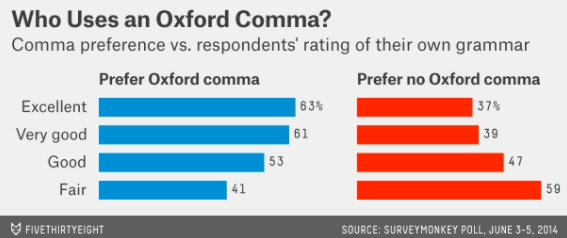
That survey also addressed an even more important grammatical issue: use of the Oxford comma. Survey participants were asked to give their opinion about which sentence is more grammatically correct:
It’s important for a person to be honest, kind and loyal.
It’s important for a person to be honest, kind, and loyal.
The survey results were that 57% of respondents favored the second sentence, with the Oxford comma*, and 43% preferred the second sentence. Fivethirtyeight also reported that those who rated their own use of grammar highly tended to prefer the Oxford comma to a greater degree than those who had a lower opinion of their own grammar, as shown in this graph:
* My strong preference is for the Oxford comma. I found simply typing the first version, without the Oxford comma, to be a traumatic experience.
I enjoy thinking about these kinds of grammar issues, but then I majored in English as well as Mathematics in college. Some of the books on my shelf beside me right now include 100 Ways to Improve Your Writing* (by Gary Provost), On Writing (by Stephen King), The Sense of Style (by Steve Pinker), and Several Short Sentences about Writing (by Verlyn Klinkenburg), along with Factfulness (by Hans Rosling) and Enlightenment Now** (also by Steven Pinker).
* My favorite piece of advice from this book can be found here.
** See posts #33 and #34, titled Reveal human progress, here and here, for more about these books.
One benefit of teaching a course called Statistical Communication is that I can justify spending some time thinking about, and writing questions about, issues of grammar that appeal to me. I am curious to know what my students think about this activity and quiz. I told them that I consider this fun, but I’m not confident that many of them agree. What do you think – whosewho’s with me?
In one of my classes last week, I realized that I was dutifully following a piece of advice that I gave in a blog post more than one year ago. Because I don’t always heed my own advice, I decided that this was noteworthy enough to warrant its own blog post.
In post #33 (here), I implored statistics teachers to use data, examples, activities, and assignments that reveal human progress. I provided many examples in that post and its follow-up (here), involving things such as increasing life expectancy and decreasing poverty rates around the world over the past few decades. Ironically, the global pandemic began to disrupt all of our lives shortly after those posts appeared.
I still believe that it’s worthwhile to make students aware of data that reveal good news and human progress. I recently read some news reports that inspired me to do this. I asked students in my Statistical Communication class* to read a pre-peer-review article about an experimental vaccine for malaria (here). This vaccine for malaria has the potential for a huge, positive impact on human welfare, particularly among children in Africa**.
* See post #94 (here) for another activity that I used in this class.
** The World Health Organization estimates that more than 400,000 people died of malaria in 2019, with African children the most vulnerable group (here).
How did I try to ask good questions of my students about the malaria vaccine article? To begin with, I gave them an online, auto-graded quiz consisting of ten questions. In fact, I think you’ll get a good sense of the article just by reading my quiz questions and knowing that the correct answer is the always the first option presented here:
What is the World Health Organization’s goal for the efficacy of a malaria vaccine by the year 2030? [Options: 75%, 50%, 90%, 95%, 99%]
In what country was this study conducted? [Options: Burkina-Faso, Kenya, United Kingdom, United States, India, Sweden]
Was this an observational study or a randomized experiment? [Options: randomized experiment; observational study]
How many treatment groups were used? [Options: three, two, four, five, six]
What ages were the subjects in this study, when they were randomized into one of the treatment groups? [Options: 5-17 months, 5-17 years, 16 years and older]
How many subjects were enrolled and received at least one vaccination? [Answer: 450]
Which group was NOT blinded as to which subjects received which treatment? [Options: pharmacists, participants, participants’ families, local study team]
Which of the following was NOT studied as a possible confounder? [Options: race, gender, age group, bed net use]
Which of the following comes closest to the percentage of participants with adequate bed net use? [Options: 85%, 95%, 75%, 50%, 25%]
What was the vaccine efficacy of the high-dose treatment after one year? [Answer: 77%]
Notice that the first and last of these ten questions reveal the great promise of this vaccine.
One purpose of these quiz questions is to guide students in their reading. I don’t mind if they look at the quiz questions in advance and if they refer to the quiz questions while they are reading. Of course, I hope that my students read the full article and don’t treat this as a scavenger hunt to find the answers to my questions. But I hope that my questions point students to some of the most important take-away points from the article.
—
Another purpose of the quiz is to prepare students for our in-class discussion. I admit that I do not feel very confident with leading class discussions, particularly via zoom. Two pieces of advice that I give myself here are to ask good questions* and give students time to discuss their answers in small groups first.
* You knew this was coming.
Because this class is about statistical communication rather than statistical concepts or methods, I posed this question to guide the discussion: What elements of the study should appear in a news article for the general public about this study? In addition to providing a list of these elements, I also asked students to classify each element that they proposed into one of three categories: (1) essential, (2) helpful but not essential, (3) unnecessary.
Before I assigned students to breakout rooms to discuss this in small groups, I decided that I should first provide a few examples of what I mean by elements of the study. I gave these three:
where the study was conducted
how many subjects participated
affiliations of the researchers.
After a brief discussion, I used a zoom poll for students to vote on how they wanted to classify each of these three elements. A large majority voted that the first two items are essential. On the third item, the vote was about evenly split between the “helpful” and “unnecessary” categories. I chimed in that there were so many co-authors on the study that I would include at most the affiliation of the lead author in a news report.
Then I assigned students to discuss this question in breakout rooms with 3-4 students each. After fifteen minutes, we reconvened as a full class to discuss what they had come up with. I typed their suggestions into a file that I projected to their screens during class and then posted after class. For each element that they mentioned, we conducted a zoom poll to vote on whether the item was essential, helpful, or unnecessary. When the discussion began to lose steam, I consulted my own list that I had created before class. In both sections of the course, a few items on my list had not been mentioned by the students, so I offered them for consideration.
Some of the items that my students identified as essential included:
background information about severity and consequences of malaria
selection criteria, including ages of the participants
when the study was conducted
use of random assignment, blindness
treatments used, including for the control group
response variable studied (whether or not the person developed malaria)
percentages in each group who developed malaria
statistical significance of the results
Some elements that were identified as helpful but not essential include:
charts or graphs of the results
ethics permissions that were obtained
adverse reactions that were studied
potential confounding variables that were studied
next steps to be taken
For the last five minutes of class, I asked a different question: What are some criteria for evaluating whether a news article provides a good report for the general public about this study? I suggested that the article should include all elements that we considered to be essential. Some suggestions from my students included:
captures interest at the outset
makes case for importance
appears visually appealing
uses appropriate language for general audience
includes link to the source article
states appropriate conclusions (not over- or under-stated) from study
includes some, but not too many, specific statistics from the study
interprets values correctly
does not contain errors
That covers questions that I asked before and during class. Here’s the assignment that students are working on before our next class session: Find a news article about the malaria vaccine study that we discussed in class. Include a link to this article with your report. Identify which essential and helpful elements (as we identified in class) are included, and not included in the article. Then write a paragraph analyzing how well the article summarizes and presents the malaria vaccine study for the general public.
This malaria vaccine article could provide an worthwhile example in an introductory statistics course, as well. For example, you could discuss experimental design issues such as random assignment and double-blindness. The example also lends itself to analyzing categorical data, both descriptively and with a chi-square test to compare success proportions among three groups.
I’m fairly pleased with how this particular session of my Statistical Communication course went, for several reasons. Sometimes I feel guilty that I often present examples from before many of my students were born, so I’m delighted to focus on an article that made the news just a few weeks ago. I am also very happy to introduce students to a research study that holds promise for considerable progress about human welfare and global health. It’s very gratifying to show students that science and statistics can contribute to such hopeful developments. It’s also just plain fun to share such good news!
This guest post has been contributed by Anelise Sabbag. You can contact her at asabbag@calpoly.edu.
Anelise Sabbag is a colleague of mine in the Statistics Department at Cal Poly – San Luis Obispo. She earned her Ph.D. in the field of statistics education at the University of Minnesota. Anelise regularly teaches our course for prospective teachers, as well as many other statistics courses, and she also conducts research into how students learn statistics. She began teaching online, and studying how students learn effectively online, well before the pandemic forced many of us to teach remotely. I am delighted that Anelise agreed to write this guest blog post about fostering collaborative learning in online courses.
Now that we have been teaching online for a few terms, some of you might be starting to consider the possibility of teaching online occasionally in the future. Maybe you have realized that online teaching is not as bad as you feared. One of the most challenging aspects is facilitating interactions among students’ online, which you may not have had time to think about as you were forced into online teaching during a pandemic. But maybe you have time to consider this now that you are a bit more used to teaching online. So, the question that I address in this blog post is: How can you encourage student-to-student interactions in your online asynchronous course?
This can be done in a variety of ways, through forum discussions and wiki assignments. But I would like to share with you another simple way to do this: a google doc file with a few good statistics questions and a collaborative structure. The “good questions” part seems to be pretty well covered in this blog already, so let’s explore a bit the idea of creating a collaborative structure in an assignment.
The idea of a collaborative structure is based on cooperative learning theory. The idea is to create an assignment that requires students to work in groups but also establishes positive interdependence among the students to encourage them to work together effectively. A collaborative structure starts with a common goal. That famous expression about “sinking or swimming together” is what we want students to understand. The success of the group is tied to the success of each student in the group. A common goal could be to require students to provide an answer to each of the good statistical questions you selected and inform the students that their responses will be graded as a group. The number of questions is really up to you. In my course, I ask about 7-8 questions per assignment, but because of time constraints I end up grading 3-4 of the questions. But having a collaborative assignment with one good question might be enough in your first attempt, until you figure out how much interesting information you can derive from these assignments. Then you might add more questions for your next iteration. But starting slowly always helps, right?
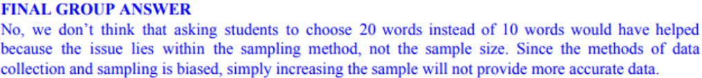
Here is an example of what I am talking about: In post #19 (here), Allan addressed the concepts of sampling bias and random sampling. The activity covered in this post asks students to read the Gettysburg Address and circle ten words as a representative sample from this passage. For each word in the sample, students are asked to record how many letters are in the word, calculate the average number of letters per word in the sample, and plot their sample average on a dotplot on the board, along with the sample averages of their classmates. Students then reflect on what they see in the dotplot and eventually conclude (or we hope they do) that this sampling method is biased. After this part of the activity, Allan suggests asking this question to students: Would asking people to circle twenty words (rather than ten) eliminate, or at least reduce, the sampling bias? I asked a very similar question in my class, and here is the final group answer for one of the groups:
This looks like a good answer, right?! It seems students are recognizing that the issue is really the sampling method and so increasing the sample size would not help. So, the students in this group were able to accomplish the shared goal of providing a strong group answer to this question.
But don’t you wish you could see the students’ thought process and interactions that led to this answer? Of course you do! At this point we have no clue about whether students worked together to get to this final answer. It could be that one student just wrote this answer and didn’t even discuss it with their group members. So, the collaborative structure of the assignment is not reflected in this final group answer. We need more!
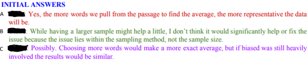
The answer I showed above is the last step of a three-step process in my collaborative assignments. Now I will tell you what happens before that. We need to create a structure in the assignment that encourages students to get to that final group answer through collaboration and discussion. We could ask them to get together on Zoom and discuss (remember that the structure here is an online asynchronous class). But we might have several issues with that approach. First, students need to find a time that they can all get together at the same time. That could already be tricky depending on the number of students in the group. Another issue we might face is student participation in this online discussion. Some students might not be willing to participate, perhaps because they are shy or maybe because they do not care. (Yeah, it is hard to admit that some students, especially in a general education course, do not really care about our beloved introductory statistics course.) So, if there is a way for students to do less work in the course, some of them will unfortunately choose that route. The issue then becomes individual accountability. Even though students are working together, we still want to hold them accountable for their individual work. So why not ask students to answer the questions individually first and then share their individual response with their group? Here are the initial answers that eventually led to the final group answer above:
Now we can see that the three students were not all on the right track initially. Student A, like many students in introductory statistics courses, might be thinking that a larger sample size leads to a representative sample. This student is most likely ignoring whether the sampling method is biased or not. Student B has the best answer compared to the other two answers. She does recognize that the issue is still the biased sampling method used. Her first comment, though, makes me want to ask a follow up question: In what way do you think increasing the sample size “might help a little”? I am hoping that this student would talk about precision, which would be great. Though she might talk about accuracy, which would not make me so happy because that is an incorrect connection (larger sample size leads to more accuracy when estimating the parameter of interest) that many students make. I think that Student C is moving toward this mistake when she says that the larger sample size would make the average more exact. This student then contradicts this first idea at the end of her sentence when stating that the results would be similar. If I could, I would ask her: How can the average be more exact and the results still be similar? By the way, I never did ask these questions as I am not “involved” in this part of the assignment. At this point, students only share the google doc file with their group members.
While asking students to provide initial answers might help students to be individually accountable, we are still stuck with the issue of students needing to find a time that they can all get together at the same time. So, why not make the discussion asynchronous? Even better, why not make this a written discussion? In this way you could get more insight into students’ thought processes. Using a google doc file can make this very straightforward. Students start by posting their initial answers in the file and sharing with their group members. Then they can have some sort of discussion about these answers to come up with a final group answer. Here is the discussion that the students had to get to final answer above:
This discussion is not as thoughtful as you might want, but it’s still interesting. The student who gave the right answer earlier is now helping the other students to understand what they might have missed. Of course, this is not the same help that a professor would give to a student, but you still see some interesting interactions. Student A, who was the one displaying worst understanding in the initial answer, seems to now be paying more attention to the sampling method, which she failed to do before. Student C also seems to be on the right track now, but this student could be just re-stating Student B’s answers. Or maybe this student finally understood that increasing the sample size will not account for the bias in the sampling method.
Of course, you are not always going to see thoughtful and encouraging discussions. Ideally, we hope that once all initial answers are provided, students will read and compare their answers, identify and correct mistakes so that they can finally end with a final group answer that is correct. The amount of interaction you see might depend on how specific your instructions are. You could require a minimum number of words in the discussion section or that every student should provide at least two contributions to the discussion.
Sometimes you might see a disappointing discussion, because students are not able to identify which answers are correct/incorrect as they are still unclear about the material. So, while students are completing this collaborative assignment, I release video(s) to help them. Please note that the statistical questions I use in these collaborative assignments are part of activities that students are required to complete individually first (and submit for grading based on completion). Usually, the activity consists of 30-40 questions, but the collaborative assignment is composed of only 7-8 of those questions. So, the videos that I release to students refer to the most important aspects of the activity and might include examples of typical mistakes students usually make. Students report that these videos are very helpful resources for them to complete these collaborative assignments. In addition to these videos, I also have “question forums” through which students can post any questions they might have about the assignments they are completing. Sometimes these also become helpful resources to students (see example below).
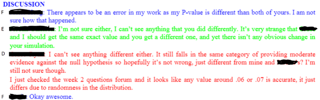
One important aspect in these assignments is to provide questions that could inspire discussion, or questions for which you think students might struggle and reach different answers. But even if students end up with similar and correct answers, you might still get some good interactions. For instance, a basic question that many of us are already asking our students is to calculate a p-value and show their work. In the example below, students noticed that they used the same correct inputs in the simulation but ended up with slightly different p-values. They were a bit stuck on this and looked at the “question forum” to get some help, where they noticed that some students already posted a question about this. At the end maybe they were able to recognize the role of random chance in their simulations.
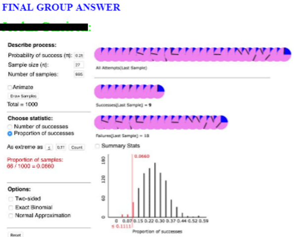
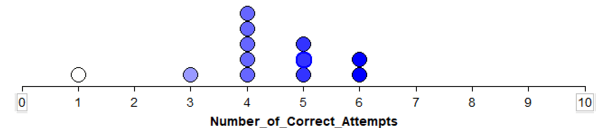
Here is another example of a collaborative assignment using one of the questions that Allan suggests in post #41 (here). When students are conducting a simulation-based analysis, we want to make sure that they know what they are doing and are not just blindly following instructions. So, we can simply ask: What does each of the 1000 dots represent? I asked a similar question in an activity that guides students in examining whether dogs understand human cues (this activity is from the textbook used in my course: Introduction to Statistical Investigations by Tintle et al). To test this, an experimenter performed some sort of gesture (pointing, bowing, looking) toward one of two cups. The researchers then saw whether the dog would go to the cup that was indicated. Students are presented with the performance of a dog named Harley, who was tested 10 times and chose the correct cup for 9 of those times. One of the earlier questions in the activity shows an example of a student (Julia) flipping a coin 10 times to simulate the process of Harley randomly choosing between the cups. For each set of 10 flips, Julia records the number of heads. She repeats this process 11 times and creates the following dotplot:
Students are then asked: Using the context of the problem, explain what a dot on the plot represents.
In this example, we see students reflecting on their own answers and also going back to the question that was asked and the information (dotplot) provided to them. Students were able to help each other differentiate between the proportion and count of success and also bring in the context of the problem to their final answer, which none of them did initially. This is an example of a group containing only two students (the third group member dropped the class). In my experience, these collaborative assignments work better in groups of 3 (which would also help with the amount of time grading), but this group was mostly successful throughout the quarter.
In my course, students are randomly put into groups at the beginning of the quarter. The first week of class is focused heavily on getting to know each other, clarifying expectation of work individually and as a group, and creating an individual and group schedule for the remainder of the quarter. These first week assignments are essential in an online course! I believe we must help students recognize that their success in an online course is tied to their organization and schedule. I also believe that these beginning “organize yourself and your group” assignments set the stage for helpful and constructive group interactions. And I believe this is why I usually do not have “group problems” in my course, and students end up working with their group through the whole quarter. The more we help the group to get to know each other and work together, the more they will help each other and learn together. To encourage positive group interactions, you could even offer them a group reward. For instance, if all students in the group do well on the individual homework at the end of the week, then everyone in the group will receive an extra credit point.
I hope this post can give you some ideas of how to provide your online students with opportunities to work together. I have high hopes that you will be pleasantly surprised with what you will see.
One of my favorite class sessions when I teach probability is the day that we study independent events. This post will feature questions that I pose to students on this topic, which (as usual) appear in italics.
I introduce conditional probability and independence with some real data that Beth Chance and I collected in 1998, when the America Film Institute unveiled a list of what they considered the top 100 American films (see the list here). Beth and I tallied up which films we had seen and produced the following table of counts:
Suppose that one of these 100 films is selected at random, meaning that each of the 100 films is equally likely to be selected.
a) What is the probability that Beth has seen the film?
b) Given the partial information that Allan has seen the film, what is the updated (conditional) probability that Beth has seen it?
c) Does learning that Allan has seen the randomly selected film change the probability that Beth has seen it? In which direction? Why might this make sense?
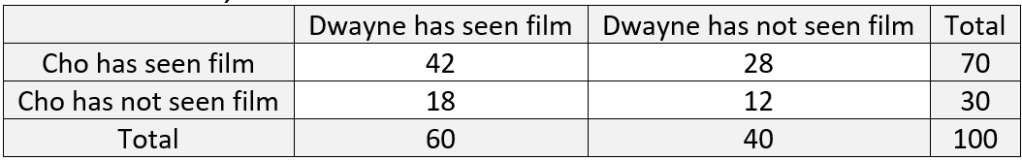
d) Repeat this analysis based on the following table (of made-up data) for two other people, Cho and Dwayne:
These probabilities are Pr(B) = 59/100 = 0.59 and Pr(B|A) = 42/48 = 0.875. Learning that Allan has seen the film increases the probability that Beth has seen it considerably. On the other hand, learning that Cho has seen the film does not change the probability that Dwayne has seen it: Pr(D) = 60/100 = 0.60 and Pr(D|C) = 42/70 =0.60.
e) In which case (Allan-Beth) or (Cho-Dwayne) would it make sense to say that the events are independent?
This question is my attempt to lead students to define the term independent events for themselves, without simply copying what I say or reading what the textbook says. Dwayne’s having seen the film is independent of Cho’s having seen it, because the probability that Dwayne has seen the film does not change upon learning that Cho has seen it. But Beth’s having seen the film is not independent of Allan’s having seen it, because her probability changes in light of that partial information about the film.
f) Based on these data, would you still say that (Allan having seen the film) and (Beth having seen the film) are dependent events, even if they never saw any films together and perhaps did not even know each other?
This question points to a fairly challenging idea for students to grasp. Probabilistic dependence does not require a literal or physical connection between the events. In this case, even if Allan and Beth did not know each other, being a similar age or having similar tastes could explain the substantial overlap in which films they have seen. Similarly, Cho and Dwayne might have watched some films together, but the data reveal that their movie-watching habits are probabilistically independent.
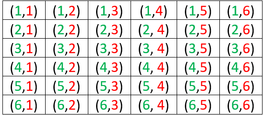
My next example gives students more practice with identifying independent and dependent events, in the most generic context imaginable: rolling a pair of fair, six-sided dice. Let’s assume that one die is green and the other red, so we can tell them apart.
Consider these four events: A = {green die lands on 6}, B = {red die lands on 5}, C = {sum equals 11}, D = {sum equals 7}. For each pair of events, determine whether or not the events are independent. Justify your answers with appropriate probability calculations.
Here is the sample space of 36 equally likely outcomes:
We know that A and B are independent events, because we assume that rolling two fair dice means to roll them independently, so the outcome for one die has no effect on the outcome for the other. The calculations are Pr(A) = 1/6, Pr(B) = 1/6, Pr(A|B) = 6/36 = 1/6, and Pr(B|A) = 6/36 = 1/6.
It makes sense that A and C are not independent, because learning that the green die lands on 6 increases the chance that the sum equals 11. The calculations are: P(C) = 2/36 = 1/18 and Pr(C|A) = 6/36 = 1/6. From the other perspective, Pr(A) = 1/6 and Pr(A|C) = 1/2, because learning that the sum is 11 leaves a 50-50 chance for whether the green die landed on 6 or 5. The events B and C are also dependent, for the same reason and with the same probabilities.
Some students are surprised to work out the probabilities and find that A and D are independent. We can calculate Pr(D) = 6/36 = 1/6 and Pr(D|A) = 1/6. This conditional probability comes from restricting our attention to the last row of the sample space, where the green die lands on 6. Even though the outcome of the green die is certainly relevant to what the sum turns out to be, the sum has a 1/6 chance of equaling 7 no matter what number the green die lands on. Similarly, B and D are also independent.
The events C and D also make an interesting case. Some students find the correct answer to be obvious, while others struggle to understand the correct answer after it’s explained to them. I like to offer this hint: If you learn that the sum equals 7, how likely is it that the sum equals 11? I want them to say that the sum certainly does not equal 11 if the sum equals 7. Then I follow up with: So, does learning that the sum equals 7 change the probability that the sum equals 11? Yes, the probability that the sum equals 11 becomes zero!* These events C and D are definitely not independent, because Pr(D) = 2/36 but Pr(D|C) = 0, which is quite different from 2/36.
* Be careful not to read this as zero-factorial**.
** I never get tired of this joke.
Next I show students that if E and F are independent events, then Pr(E and F) = Pr(E) × Pr(F). Then I provide an example in which we assume that events are independent and calculate additional probabilities based on that assumption.
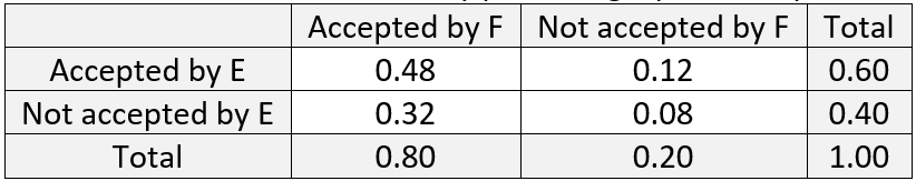
Suppose that you have applied to two internship programs E and F. Based on your research about how competitive the programs are and how strong your application is, you believe that you have a 60% chance of being accepted for program E and an 80% chance of being accepted for program F. Assume that your acceptance into one program is independent of your acceptance into the other program.
a) What is the probability that you will be accepted by both programs?
b) What is the probability that you will be accepted by at least one of the two programs? Show two different ways to calculate this.
Part (a) is as simple as they come: Pr(E and F) = Pr(E) × Pr(F) = 0.6 × 0.8 = 0.48*. For part (b), we could use the addition rule: Pr(E or F) = Pr(E) + Pr(F) – Pr(E and F) = 0.6 + 0.8 – 0.48 = 0.92. We could also use the complement rule and the multiplication rule for independent events, because complements of independent events are also independent: Pr(E or F) = 1 – Pr(not E and not F) = 1 – Pr(not E) × Pr(not F) = 1 – 0.4 × 0.2 = 0.92. I like to specify that students should solve this in two different ways. I go on to encourage them to develop a habit of looking for multiple ways to solve probability problems in general. Students could also solve this by producing a probability table:
* You probably noticed that I was a bit lax with notation here. I am using E to denote the event that you are accepted into program E. Depending on the student audience, I might or might not emphasize this point.
Next I mention that the multiplication rule generalizes to any number of independent events. Then I ask: Now suppose that you also apply to programs G and H, for which you believe your probabilities of acceptance are 0.7 and 0.2, respectively. Continue to assume that all acceptance decisions are independent of all others.
c) What is the probability that you will be accepted by all four programs? Is this pretty unlikely?
d) What is the probability that you will be accepted by at least one of the four programs? Is this very likely?
Again part (c) is quite straightforward: Pr(E and F and G and H) = Pr(E) × Pr(F) × Pr(G) × Pr(H) = 0.6 × 0.8 × 0.7 × 0.2 = 0.0672. This is pretty unlikely, less than a 7% chance, largely because of applying to very competitive program H. Part (d) provides much better news: Pr(E or F or G or H) = 1 – Pr(not E and not F and not G and not H) = 1 – Pr(not E) × Pr(not F) × Pr(not G) × Pr(not H) = 1 – 0.4 × 0.2 × 0.3 × 0.8 = 0.9808. You have a very good chance, better than 98%, of being accepted into at least one program.
e) Explain why the assumption of independence is probably not reasonable in this situation.
Even though the people who administer these scholarship programs would not be comparing notes on applicants or colluding in any way, learning that you were accepted into one program probably increases the probability that you’ll be accepted by another, because they probably have similar criteria and standards. It’s plausible to believe that learning that you were accepted by one school makes it more likely that you’ll be accepted by the other, as compared to your uncertainty before learning about your acceptance to the first school. This means that the calculations we’ve done should not be taken too seriously, because they relied completely on the assumption of independence.
Next I ask students to consider a context in which independence is much more reasonable to assume and justify:
Suppose that every day you play a lottery game in which a three-digit number is randomly selected. Your probability of winning for each day is 1/1000.
a) Is it reasonable to assume that whether you win or lose is independent from day to day? Explain.
b) Determine the probability that you win at least once in a 7-day week. Report your answer with five decimal places. Also explain why this probability is not exactly equal to 7/1000.
c) Determine the probability that you win at least once in a 365-day year.
d) Suppose that your friend says that because there are only 1000 three-digit numbers, you’re guaranteed to win once if you play for 1000 days. How would you respond?
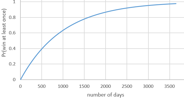
e) Express the probability of winning at least once as a function of the number of days that you play. Also produce a graph of this function, from 1 to 3652 days (about 10 years). Describe the function’s behavior.
f) For how many days would you have to play in order to have at least a 90% chance of winning at least once? How many years is this?
g) Suppose that the lottery game costs $1 to play and pays $500 when you win. If you were to play for that many days (your answer to the previous part), is it likely that you would end up with more or less money than you started with?
Because the three-digit lottery number is selected at random each day, whether or not you win on any given day does not affect the probability of winning on any other day, so your results are independent from day to day.
We will use the complement rule and the multiplication rule for independent events throughout this example: Pr(win at least once) = 1 – Pr(lose every day) = 1 – (0.999)n, where n represents the number of days. For a 7-day week in part (b), this produces Pr(win at least once) = 1 – (0.999)7 ≈ 0.00698. Notice that this is very slightly less than 7/1000, which is what we would get if we added 0.001 to itself for the seven days. Adding these probabilities does not (quite) work because the events are not mutually exclusive, because it’s possible that you could win on more than one day. But it’s extremely unlikely that you would win on more than one day, so this probability is quite close to 0.007. I specifically asked students to report five decimal places in their answer just to see that the probability is not exactly 0.007*.
* I like to refer to this as a James Bond probability.
For the 365-day year in part (c), we find: Pr(win at least once) = 1 – (0.999)365 ≈ 0.306. The friend’s argument in part (d) about being guaranteed to win if you play for 1000 days is not legitimate, because it’s certainly possible that you would lose on all 1000 days. In fact, that unhappy prospect is not terribly unlikely: Pr(win at least once) = 1 – (0.999)1000 ≈ 0.632 is greater than one-half but much closer to one-half than to one!*
* Feel free to read this as one-factorial.
Here’s the graph requested in part (e) for the function Pr(win at least once) = 1 – (0.999)n:
This function is increasing, of course, because your probability of winning at least once increases as the number of days increases. But the graph is concave down, meaning that the rate of increase gradually decreases as time goes on. The probability of winning at least once reaches 0.974 after 10 years of playing every day.
Part (f) asks us to solve the inequality 1 – (0.999)n ≥ 0.9. We can see from the graph that the number of days n needs to be between 2000 and 2500. Examining the spreadsheet in which I performed the calculations and produced the graph reveals that we need n ≥ 2302 days in order to have at least a 90% chance of winning at least once. This is equivalent to 2302/365.25 ≈ 6.3 years. If you’d like your students to work with logarithms, you could ask them to solve the inequality analytically. Taking the log of both sides of (0.999)n ≤ 0.1 and solving, remembering to flip the inequality when diving by a negative number, gives: n ≥ log(0.1) / log(0.999) ≈ 2301.434 days.
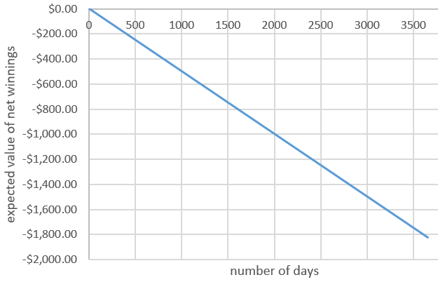
I included part (g) just to make sure that students realize that winning at least once does not mean coming out ahead of where you started financially. At this point of the course, we have not yet studied random variables and expected values, but I give students a preview of coming attractions by showing this graph of the expected value of your net winnings as a function of the number of days that you play*:
* The expected value of net winnings for one day is (-1)(0.999) + (500)(.001) = -0.499, so the expected value of net winnings after n days is -0.499 × n.
I still have not gotten to my favorite example for independence day, but this post is already long enough. That example will have to wait for part 2 of this post, which will not be independent of this first part in any sense of the word.
This weekly blog provides ideas, examples, activities, assessments, and advice for teaching introductory statistics, all based on a three-word teaching philosophy: Ask good questions.
Each post aims to be both practical and thought-provoking.
See the first blog post (here) for answers to ten questions about this blog.