#2 My favorite question

This blog is about asking good questions to teach introductory statistics, so let me tell you about my all-time favorite question.  I want to emphasize from the outset that I had nothing to do with writing it. I’m just a big fan.

I am referring to question #6, called an investigative task, on the 2009 AP Statistics exam.  I’ll show you the question piece-by-piece, snipped from the College Board website. You can find this question and many other released AP Statistics exams here.

Here’s how the question begins:

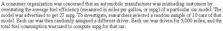
Oh dear, I have to admit that this is an inauspicious start.  Frankly, I think this a boring, generic context for a statistics question.  Even worse, there’s no mention of real data. What’s so great about this? Nothing at all, but please read on …

I think this is a fine question, but I admit that it’s a fairly routine one. Describing the parameter in a study is an important step, and I suspect that students find this much more challenging than many instructors realize.  I would call this an adequate question, perhaps a good question, certainly not a great question. So, I don’t blame you if you’re wondering why this is my all-time favorite question.  Please read on …

Now we’re getting somewhere.  I think this is pretty clever: presenting students with a statistic that they have almost certainly never encountered before, and asking them to figure out something about the unknown statistic based on what they know.  The question is not particularly hard, but it does ask students to apply something they know to a new situation. Students should realize that right-skewed distributions tend to have a larger mean than median, so the ratio mean/median should be greater than 1 with these data.

Part (b) also helps students to prepare for what comes next …

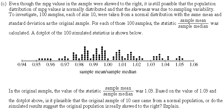
Now we’re talking!  I think part (c) makes this a great question.  To answer this part well, students have to understand the reasoning process of statistical significance, and they have to apply that reasoning process in a situation that they have almost surely never encountered or even thought about: making an inference about the symmetry or skewness of a population distribution.  This is extremely challenging, but I think this assesses something very important: whether students can apply what they have learned to a novel situation that goes a bit beyond what they studied.

Notice that this question does not use words such as hypothesis or test or reject or strength of evidence or p-value.  The key word in the question is plausible.  Students have to realize that the simulation analysis presented allows them to assess the plausibility of the assumption underlying the simulation: that the population follows a normal distribution.  Then they need to recognize that they can assess plausibility by seeing whether the observed value of the sample statistic is unusual in the simulated (null) distribution of that statistic. It turns out that the observed value of the mean/median ratio (1.03) is not very unusual in the simulated (null) distribution, because 14/100 of the simulated samples produced a statistic more extreme than the observed sample value.  Therefore, students should conclude that the simulation analysis reveals that a normally distributed population could plausibly have produced the observed sample.

A common student error is not recognizing the crucial role that the observed value (1.03) of the statistic plays.  More specifically, two common student errors are:

• Commenting that the simulated distribution is roughly symmetric, and concluding that it’s plausible that the population distribution is normal.  Students who make this error are failing to notice the distinction between the simulated distribution of sample statistics and the population distribution of mpg values.
• Commenting that the simulated distribution of sample statistics is centered around the value 1, which is the expected value of the statistic from a normal population, and concluding that it’s plausible that the population distribution is normal.  Students who make this error are failing to realize that the simulation assumed a normal population in the first place, which is why the distribution of simulated sample statistics is centered around the value 1.

If this question ended here, it would be one of my all-time favorites.  But it doesn’t end here. There’s a fourth part, which catapults this question into the exalted status of my all-time favorite.  Once again (and for the last time!), please read on…

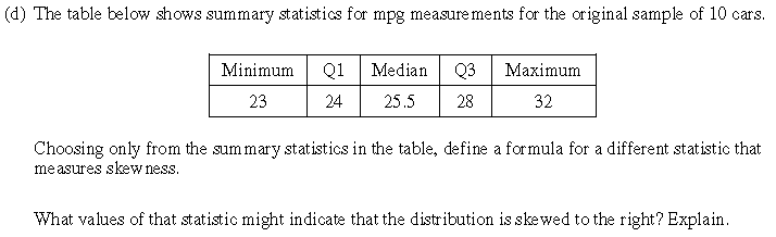
Wow, look at what’s happening here!  Students are being told that they don’t have to restrict their attention to common statistics that they have been taught.  Rather, this question asks students to exercise their intellectual power to create their own statistic! Moreover, they should know enough to predict how their statistic will behave in a certain situation (namely, a right-skewed distribution).  This part of the question not only asks students to synthesize and apply what they have learned, but it also invites students to exercise an intellectual capability that they probably did not even realized they possess. Some common (good) answers from students include the following statistics, both of which should take a value greater than 1 with a right-skewed distribution:

• (maximum – median) / (median – minimum)
• (upper quartile – median) / (median – lower quartile)

There you have it: my all-time favorite question from an introductory statistics exam.  I encourage you to ask this question, or some variation of it*, of your students. I suggest asking this in a low-stakes setting and then discussing it with students afterward.  Encourage them to realize that the reasoning processes they learn in class can be applied to new situations that they have not explicitly studied, and also help them to recognize that they are developing the intellectual power to create new analyses of their own.

* Even though this is my all-time favorite question, I suggest three revisions related to part (c).  First, I would provide students with sample values of the mean and median and ask them to calculate the value of the ratio for themselves.  I think this small extra step might help some students to realize the importance of seeing where the observed value of the statistic falls in the simulated distribution.  Second, I recommend altering the sample data a bit to make the observed value of the sample statistic fall quite far out in the tail of the simulated (null) distribution of the statistic.  This would lead to rejecting the plausibility of a normally distributed population in favor of concluding that the population distribution was right-skewed.  I think this conclusion might be a bit easier for students to recognize, while still assessing whether students understand how to draw an appropriate conclusion from the simulation analysis.  Third, I would prefer to use 1000 or 10,000 repetitions for the simulation, which would require using a histogram rather than a dotplot for the display.

P.S. I mentioned at the top that I had nothing to do with writing this question.  Three people who played a large role in writing it and developing a rubric for grading it were Bob Taylor, Chris Franklin, and Josh Tabor.  They all served on the Test Development Committee for AP Statistics at the time. Bob chaired the committee, Chris served as Chief Reader, and Josh was the Question Leader for the grading of this question. Josh also wrote a JSE article (here) that analyzed various choices for the skewness statistic in part (d).