#21 Twenty final exam questions

My mantra of “ask good questions” applies to exams as well as in-class learning activities.  This week I present and discuss twenty multiple-choice questions that I have used on final exams.  All of these questions are conceptual in nature.  They require no calculations, they do not refer to actual studies, and they do not make use of real data.  I certainly do not intend these questions to comprise a complete exam; I strongly recommend asking many free-response questions based on real data and genuine studies as well.

At the end of this post I provide a link to a file containing these twenty questions, in case that facilitates using them with your students.  Correct answers are discussed throughout and also reported at the end.

---

I like to think that this question assesses some basic level of understanding, but frankly I’m not sure.  Do students ever say that a standard deviation and a p-value can sometimes be negative?  Not often, but yes.  Do I question my career choice when I read those responses?  Not often, but yes.

---

I think it’s valuable to ask students to apply what they’ve learned to a new situation or a bew statistic.  This question is not nearly as good for this goal as my favorite question (see post #2 here), but I think this assesses something worthwhile.  The questions about resistance are fairly straightforward.  The mid-hinge is resistant because it relies only on quartiles, but the mid-range is very non-resistant because it depends completely on the most extreme values.  Both of these statistics are measures of center.  This is challenging for many students, perhaps because they have seen that the difference between the maximum and minimum, and the difference between the quartiles, are measures of variability.  One way to convince students of this is to point out that adding a constant to every value in the dataset (in other words, shifting all of the data values by the same amount) would cause the mid-hinge and mid-range to increase (or shift) by exactly that constant.

---

This question should be very easy for all students, but some struggle.  The question boils down to: If the sum of values equals zero, does the mean have to equal zero, and does the median have to equal zero?  The answer is yes to the first, because the mean is calculated as the sum divided by the number of values.  But the answer is no to the second, as seen in this counterexample where the mean is 0 but the median is not: -20, 5, 15.  The fact that this question is stated about residuals is completely irrelevant to answering the question, but the mention of residuals leads some students to think in unhelpful directions.

I sometimes ask an open-ended version of this question where I ask students to provide a counter-example if their answer is no.

---

This question has been extremely challenging for my students.  I used to ask it without providing options, and the most common response was “the same.”  That’s right: Many students did not realize that they should provide a number when asked for the value of a correlation coefficient.  Among these options, it’s very discouraging when a student selects -5, apparently not knowing that a correlation coefficient needs to be between -1 and +1 (inclusive), but this answer is tempting to some students because of the “5 points lower” wording in the question.  Another commonly selected wrong answer is -1.  I think students who answer -1 realize that the data would fall on a perfectly straight line, so the correlation coefficient must be -1 or +1, but the “lower” language fools them into thinking that the association is negative.

I sometimes offer a hint, advising students to start by drawing a sketch of some hypothetical data that satisfy the description.  I have also started to ask and discuss this question in class when we first study correlation, and then include the exact same question on the final exam.  This has improved students’ performance, but many still struggle.

---

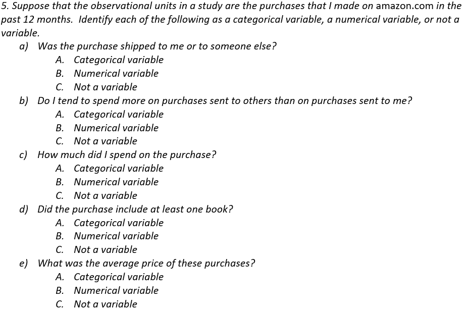
Most students correctly identify (a) and (d) as categorical variables and (c) as a numerical variable.  The most challenging parts are (b) and (e), which are not variables for these observational units.  I try to emphasize that variables are things that can be recorded for each observational unit, not an overall question or measure that pertains to the entire dataset.

---

I started asking this question after I noticed that some of my students believe that conducting a randomized experiment always justifies drawing a cause-and-effect conclusion, regardless of how the data turn out!  The good news is that very few students give answer A.  The bad news is that more than a few give answer C.

---

Some students take the “correlation does not imply causation” maxim to an inappropriate higher level by believing that “correlation implies no causation.”  Of course, I want them to know that a strong correlation does not establish a cause-and-effect relationship but also does not preclude that possibility.

---

I often ask this question as a calculation to be performed in my courses for mathematically inclined students.  To calculate the correct percentage, note that Brad will get 70% right because he knows the answer, and he’ll guess correctly on 1/3 of the other 30%.  So, his long-run percentage correct will be 70% + 1/3(30%) = 80%.

When I ask for this calculation, I’ve been surprised by students giving an answer less than 70%.  I understand that mistakes happen, of course, or that a student would not know how to solve this, but I can’t understand why they wouldn’t realize immediately that the answer has to be larger than 70%.  I decided to ask this multiple-choice version of the question, which does not require a numerical answer or any calculation.  I’m still surprised that a few students get this wrong.

---

This is essentially the same question as I asked in post #16 (here) about whether the percentage of American households with a pet dog plus the percentage with a pet cat equals the percentage with either a pet dog or a pet cat.  Adding these percentages is not legitimate because the events are not mutually exclusive: It’s possible that it could rain on both Saturday and Sunday.  I hope that choosing 70% and 30% as the percentages is helpful to students, who might be tipped off by the 100% value that something must be wrong because rain cannot be certain.

It might be interesting to ask this question with percentages of 70% and 40%, and also with percentages of 60% and 30%.  I hope that the version with 70% and 40% would be easier, because all students should recognize that there could not be a 110% chance of rain.  I suspect that the version with 60% and 30% would be harder, because it might be more tempting to see 90% as a reasonable chance.

---

The main point here is that you cannot just take the average of 80% and 40%, because the group sizes are not the same.  Because there are many more students than faculty, the overall percentage will be much closer to the student percentage of 80%, so the correct answer is that the overall percentage would be more than 60%.

---

The goal here is to assess whether students realize that a probability such as 0.5 refers to a long-run proportion and does not necessarily hold in the short-run.  A sample size of two children definitely falls into the short-run and not long-run category, so it’s not guaranteed or even very likely to have one child of each sex.

A student does not need to enumerate the sample space and calculate the exact probability to answer this question correctly.  The sample space of four equally likely outcomes is {B1B2, B1G2, G1B2, G1G2}, so the probability of having one child of each sex is indeed 2/4 = 0.5.  But a student only needs to realize that this event is neither very likely nor very unlikely in order to answer correctly.  In fact, even if a student has the misconception that the three outcomes {2 boys, 2 girls, 1 of each} are equally likely, so they think the probability is 1/3, they should still give the correct answer of C.

---

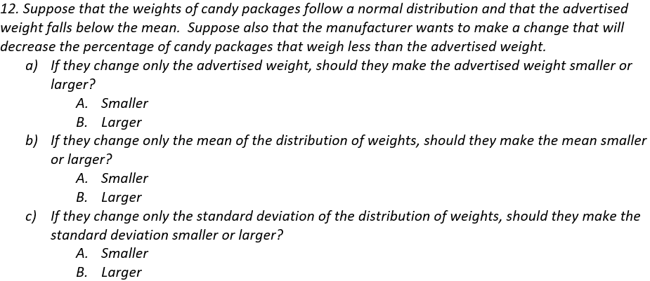
Students expect to perform normal distribution calculations after they read the first sentence.  But they cannot do this, because the mean and standard deviation are not provided.  For that matter, we also don’t know the value of the advertised weight.  Students are left with no option but to think things through.  I hope that they’ll remember and follow the advice that I give for any question involving normal distributions: Start with a sketch!

Part (a) can be answered without ever having taken a statistics course.  To reduce the percentage of packages that weigh less than advertised, without changing the mean or standard deviation, the manufacturer would need to decrease the advertised weight.

To answer part (b), students should realize that decreasing the percentage of underweight packages would require putting more candy in each package, so the mean of the distribution of weights would need to increase.

Part (c) is the most challenging part.  Decreasing the percentage of underweight packages, without changing the advertised weight or the mean, would require a taller and skinnier normal curve.  So, the standard deviation of the weights would need to decrease.

---

Most students get this wrong by answering yes.  These students have missed the whole point of the Central Limit Theorem (CLT), which describes the distribution of the sample mean.  Many students believe that whenever a sample size reaches 30 or more, that guarantees an approximately normal distribution.  Of what?  They don’t give that question any thought.  They mistakenly believe that the CLT simply guarantees a normal distribution when n ≥ 30.

I usually ask for an explanation along with a yes/no answer here.  But the explanation is almost always the same, boiling down to: Yes, because n ≥ 30.  Some students do give a very good answer, which demonstrates that they’ve learned something important (and also gives me much pleasure).  I think this question helps to identify students with a very strong understanding of the CLT from those with a less strong understanding.

You could ask a version of this question that does not refer to the Central Limit Theorem by asking: Does the sample size of 200 houses establish that …

---

This is one of my very favorite questions, which I ask on almost every final exam.  I think this is a very important idea for students to understand.  But my students perform very poorly on this question that I like so much.  Not many give the correct answer (B, 1000), and many think that the answer is 100,000 or more.

It’s fine for students to perform a sample size calculation to answer this question, but that’s not my intent.  I hope that they will have noticed that many examples in the course involved surveys with about 1000 people and that the margin-of-error turned out to be in the ballpark of 3 percentage points.

Unfortunately, many students are misled by the 325 million number that appears in the first sentence of the question.  The population size is not relevant here.  Margin-of-error depends critically on sample size but hardly at all on population size, as long as the population is much larger than the sample.  A sample size of 1000 people has the same margin-of-error whether the population of interest is all Americans or all New Zealanders or all residents of San Luis Obispo.

I suppose you could argue that I am deliberately misleading students by leading off with an irrelevant piece of information, but that’s precisely what’s being assessed: Do they realize that the population size is irrelevant here?  It’s quite remarkable that a sample size of 1000 is sufficient to obtain a margin-of-error of only 3.5 percentage points in a population as numerous as the United States.  One of my principal goals in the course is for students to appreciate the wonder of random sampling!

I sometimes give half-credit to answers of 100 and 10,000, because they are somewhat in the ballpark.  On the opposite extreme, I am tempted to deduct 2 points (even on a 1-point question!) when a student answers 1,000,000 or 10,000,000.

---

This question is about as straight-forward as they come, and my students generally do well.  Some of the questions above are quite challenging, so it’s good to include some easier ones as well.

---

This is another straightforward one on which my students do well.  I hope that the answer to this question is second-nature to students by the end of the course, and I like to think that they silently thank me for the easy point when they read this question.

---

You might be expecting me to say that this one is also straight-forward, but it is always more problematic for students than I anticipate.  Maybe some students out-smart themselves by applying an exam-testing strategy that cautions against giving the same answer for both parts of a two-part question.

---

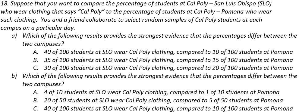
Part (a) is very clear-cut.  In fact, this is another question for which there’s no need to have ever set foot in a statistics classroom to answer correctly.  All that’s needed is to look for the result with the biggest difference between the success proportions in the two groups.

It does help to have been in a statistics classroom for part (b), although many students have correct intuition that larger sample sizes produce stronger evidence of a difference between the groups, when the difference in success proportions is the same.

---

I like questions about hypothesis tests and confidence intervals providing complementary and consistent results.  In this case students need to realize that the p-value is greater than 0.05, so the difference in the groups means is not statistically significant at the .05 level, so a 95% confidence interval for the difference in population means should include both positive and negative values (and zero).

---

This is another example of asking students to think through a statistic that they may not have encountered in class.  They should recognize that a relative risk greater than one indicates that one group has a higher success proportion than the other.  In this case, a confidence interval consisting entirely of values greater than one provides strong evidence that the success proportions differ between the two groups.

---

Because this is the post #21 in this blog series, I will include a twenty-first question for extra credit*.  Be forewarned that this is not really a statistics question, and it does not align with any conventional learning objective for a statistics course.

* I rarely offer extra credit to my students, but I happily extend this opportunity to blog readers.

I mentioned in post #8 (here) that this percentage has halved and that only 5% of a sample of Americans gave the correct answer.  Hans Rosling liked to point out that this represents a far worse understanding than pure ignorance, which would suggest that one-third would answer correctly.  Of course, knowing this fact is not a learning objective of an introductory statistics course, but I truly hope that statistics teachers can lead their students to learn about the world by presenting real data on many topics.  Later I will write a blog post arguing that statistics teachers can present data that help to make students aware of many measurable ways in which the world is becoming a better and better place.

---

P.S. More information for Rosling’s claim and survey data about the global extreme poverty rate (question #21) can be found here and here and here.

P.P.S. I thank Beth Chance for introducing me question #14 above (about the sample size needed to obtain a reasonable margin-of-error for the population of all U.S. residents).  Beth tells me that she borrowed this question from Tom Moore, so I thank him also.

I also thank Beth and Tom for kindly serving as two reviewers who very read drafts of my blog posts and offer many helpful suggestions for improvement before I post them.

Speaking of giving thanks, to those in the U.S. who read this during the week that it is posted, let me wish you a Happy Thanksgiving!

To all who are reading this in whatever country and at whatever time: Please accept my sincere thanks for taking the time to follow this blog.

P.P.P.S. Answers to these questions are: 1a) A, 1b) A, 1c) B, 1d) B, 1e) A; 2a) A, 2b) A, 2c) B, 2d) A; 3a) A, 3b) B; 4) F; 5a) A, 5b) C, 5c) B, 5d) A, 5e) C; 6) B; 7) C; 8) C; 9) B; 10) A; 11) C; 12a) A, 12b) B, 12c) A; 13) B; 14) B; 15) A; 16) C; 17a) A, 17b) A; 18a) A, 18b) C; 19) B; 20) B; 21) C.

A Word file with these twenty questions, which you may use to copy/paste or modify questions for use with your students, can be found here: