Skip to content

Archive for

#74 A sneaky quiz

Last summer I participated as a student in an online course for the first time.  The topic was how to teach an online course.  The course was delivered asynchronously, but it was not self-paced because there were regular due dates on assignments.  Somewhat to my embarrassment, I found that I was highly motivated by the assignments and those due dates.

As I have been teaching my own students online this term, I decided to give even more quizzes than usual to motivate my students to keep up.  For each topic that we have studied, I have given a handout quiz and an application quiz.  The handout quizzes have often asked the same questions that we answered as we worked through the handout, while the application quizzes have asked students to apply what they learned to a new study or situation.  As long as a student attended one of my live zoom sessions or watched the videos that I prepared, and paid a modest amount of attention, they should have done very well on the handout quizzes.  I even allowed two attempts on these handout quizzes, recording the average score.


My final class meeting of the term occurred on Monday of Thanksgiving week.  I told my students in advance that we would not study new material on that day.  Instead I provided them with practice questions about identifying which inference procedure to apply for a particular question.  As this is the first course in a two-course sequence, and we spent about half of the term studying probability, we have only studied inference for a single mean or a single proportion.  Here’s how I summarized things at the start of the handout for this class:

  • Statistical inference draws a conclusion (i.e., infers something) about a population parameter based on a sample statistic. 
    • A confidence interval estimates the value of a parameter with a range of values.
      • A population proportion π can be estimated with a z-interval.
      • A population mean μ can be estimated with a t-interval.
    • A hypothesis test assesses the plausibility of a particular claim about the parameter.
      • A claim about a population proportion π can be tested with a z-test.
      • A claim about a population mean μ can be tested with a t-test.

The instructions that I provided for the task were: For each of the following research questions, identify which of these four inference procedures would be appropriate.  Furthermore, if the research question calls for a hypothesis test, state the appropriate null and alternative hypotheses.  If the research question calls for a confidence interval, clearly identify the parameter to be estimated.

The ten questions that we analyzed were:

  • a) How many hours does a full-time Cal Poly student spend studying, per week, on average?
  • b) Does a full-time Cal Poly student spend an average of more than 25 hours per week studying?
  • c) Does the percentage of full-time Cal Poly students who were born in California differ from 80%?
  • d) What proportion of full-time Cal Poly students were born in California?
  • e) What proportion of people with a driver’s license in California have indicated a willingness to be an organ donor?
  • f) Have less than two-thirds of all people with a driver’s license in California indicated a willingness to be an organ donor?
  • g) What is the price of an average transaction at the Subway on campus?
  • h) What proportion of transactions at the Subway on campus include a soft drink?
  • i) Do most transactions at the Subway on campus include a soft drink?
  • j) Do weekday employees at a company take sick days disproportionately often on Mondays and Fridays?

We worked through the first four of these together.  I advised students to start by identifying the observational units, variable, and type of variable for each question.  I emphasized that deciding whether the parameter is a mean or a proportion boils down to determining whether the variable is numerical or categorical.  I also admitted that the question itself often contains a key (giveaway) word, such as average in parts (a) and (b), percentage in (c), and proportion in (d).

Next I asked students to discuss parts (e)-(j) together in zoom breakout rooms of 4-5 students per group.  Then we came back together to discuss these.  I pointed out that questions (f) and (i) do not use a giveaway word, so they require more careful thought.  Students need to realize that the variable in (f) is whether or not the person has indicated a willingness to be an organ donor, which is categorical, so the parameter is the proportion of all people with a California driver’s license who have indicated such a willingness.  The word most carries a lot of weight in (i), revealing that the alternative hypothesis is that the proportion of all Subway transactions that include a soft drink is greater than one-half.

Question (j) is a favorite of mine. Its impetus is an old* Dilbert cartoon, available here.  The joke is that the pointy-haired boss expresses outrage upon learning that two-fifths of all sick days at his company are taken on Mondays and Fridays.  The observational units are sick days, and the variable is whether or not the sick day was taken on Monday or Friday.  The null hypothesis asserts that two-fifths of all sick days are taken on Monday or Friday, which is what would be expected if sick days were not being mis-used to produce long weekends.  The alternative hypothesis is that more than two-fifths of all sick days are taken on Monday or Friday.

* I just realized that very few, if any, of my students were alive when this particular cartoon appeared in 1996.  Hmm, I wonder if my university’s special incentive to take early retirement is still available.


The title of this post promised something sneaky.  You might be thinking that unless sneaky has been redefined as boring, what you’ve read so far does not even come close.  Please keep reading …

I have mentioned before that my course this term is asynchronous, even though I strongly encourage students to attend my optional live zoom sessions on MWF mornings.  Because of the asynchronous listing, I feel obligated to make videos to accompany the handouts for the students who cannot, or choose not to, attend the live sessions.  These videos show me working through the examples in the handout.  I always begin by saying something like: I strongly encourage you to pause the video, answer the handout questions on your own first, and then resume the video to watch my discussion of the questions.  The videos usually show me writing answers directly in the handout file, especially when performing calculations. 

But this time I purposefully did not write on the handout for the video recording.  Instead I only talked about the ten questions (a) – (j).  For the students who ignored my advice to answer the questions for themselves before watching the video, I wanted them at a minimum to take their own notes based on what I was saying.  I hope that active listening and writing might have activated their learning to some extent.

That’s a bit of sneakiness on my part, but that does not constitute the sneaky quiz mentioned in the title of this post.


Most of my handout quiz questions throughout this term have repeated questions that were asked directly in the handout.  But this time students could not answer questions on the handout quiz merely by copying answers from their notes.  Here are the quiz questions:

  1. For how many of the ten questions in this handout are Cal Poly students the observational units?
  2. How many of the ten questions in this handout involve a categorical variable?
  3. How many of the ten questions in this handout involve inference for a population mean?
  4. How many of the ten questions in this handout ask for a confidence interval?
  5. How many of the ten questions in this handout ask for a hypothesis test with a two-sided alternative hypothesis?

I hope that this sneaky approach of mine forced students to review their notes and also reinforced some ideas about how to decide on an inference method.  I hope that these quiz questions reminded students, perhaps sub-consciously, to think about the observational units (question #1), the type of variable (#2), the parameter (#3), whether the question calls for a confidence interval or hypothesis test (#4), and whether an alternative hypothesis is one- or two-sided (#5).

My writing teachers from college might be disappointed that my previous two sentences both began with “I hope …”  Nevertheless, I return to that construction once more for my conclusion: I hope you agree that sneakiness is forgivable, perhaps even desirable, as a pedagogical strategy when the intent is to prompt student to think without their realizing it.

#73 No notes needed

My exams have been open-book, open-notes for as long as I can remember.  I tell students from the outset that they should focus on understanding rather than memorization, and I think they take comfort in knowing that they can look up formulas and definitions during exams.

As we approach the end of the fall term*, I have often told students that some terms, symbols, and facts should have become so familiar that they need not refer to their notes, even though they never set out to memorize the term, symbol, or fact.

* I am teaching the first in a two-course sequence for business majors.  We study inference for a single mean and for a single proportion at the end of the course.  The next course will begin with inference for comparing two groups.

For this blog post I decided to make a list of things that I want students to know without looking at their notes*.  In the spirit of fairness, I am going to do this without looking at any of my course notes.  In the spirit of fun, I encourage you to compile your own list before reading mine.

* This is very different from my list of thirteen important topics for students to learn. See post #52, here.


  1. The term observational unit
  2. The term variable
  3. The term categorical variable
  4. The term numerical variable
  5. The term explanatory variable
  6. The term response variable

These are the building blocks of designing a study, analyzing data, and drawing conclusions.  I don’t want my students to memorize definitions for these terms, but I ask about these so often* that I hope they can answer my questions without looking anything up.

* See post #11, Repeat after me, here.

  1. The symbol n

If students need to look up in their notes that n is our symbol for sample size, then they’re missing out on a lot.

  1. The term population
  2. The term sample
  3. The term parameter
  4. The term statistic

Again, I don’t want my students to memorize definitions of these terms, and I certainly won’t ask them to define these on an exam.  But I also don’t want students to have to stop and look up the definitions whenever they encounter these words.  In the last week or two, I have often said something like “remember that statistical inference is about inferring something about a population parameter based on a sample statistic,” and I sure don’t want students to need to look up those four terms in a glossary to understand my point.

  1. The symbol p-hat
  2. The symbol x-bar
  3. The symbol π
  4. The symbol μ

I have told my students several times in the past few weeks that understanding what these symbols mean needs to be second-nature for them.  It’s hard enough to understand a statement such as E(X-bar) = μ without having to look up what each symbol means.  I agree that we can and should express this result in words as well as symbols: If you select a very large number of random samples from a population, then the average of the sample averages will be very close to the population average.  But that’s a lot of words, and it’s very handy to use symbols.  I was very tempted to include the symbols σ and s on this list also.

  1. The term random sampling
  2. The term random assignment
  3. The term confounding variable

As I’ve written before*, I really want students to understand the difference between random sampling and random assignment.  In particular, I’d like students to understand the different kinds of conclusions that follow from these different uses of randomness.  Random sampling allows for findings about the sample to be generalized to the population, and random assignment opens the door to drawing cause-and-effect conclusions.  Confounding variables in observational studies provide an alternative to cause-and-effect explanations.  I hope that students learn these ideas well enough that they think of them as they read about statistical studies in their everyday lives.  Of course, I know that they will not refer to their notes from my class as they go about their everyday lives.

* See posts #19 and #20, Lincoln and Mandela, here and here.

  1. How to calculate an average

I always tell my students that they do not need to memorize formulas.  But I can expect them to know that calculating an average involves adding the values and dividing by the number of values, right?  I’d also like students to know that the median is the ordered value in position (n+1)/2, but that looks like a formula, so I’ll leave that off this list.

  1. The idea that standard deviation is a measure of variability

I do not expect my students to know the formula for calculating standard deviation, and I rarely ask them to calculate a standard deviation by hand.  But I do want them to know, without referring to their notes, that a larger standard deviation indicates more variability.

  1. How to calculate proportions (marginal, conditional, joint) from a two-way table of counts

My students have performed these calculations when analyzing categorical data and also for calculating conditional probabilities.  I hope that they feel confident with such calculations without using their notes.

  1. The idea that a difference between two percentages is not a percentage difference.

I don’t care if students need to look up how to calculate a percentage difference, but I do want them to know that that a difference in percentage points is not the same as a percent difference.  I don’t mean that I want to them to be able to state that fact, but I want them to recognize it when they encounter it.  For example, I’d like student to realize that increasing your success rate from 10% to 15% is not a 5% improvement in the success rate*.

* I wrote an entire essay about this in post #28, A pervasive pet peeve, here.

  1. How to interpret a z-score
  2. How to calculate a z-score

Perhaps I am violating my policy about not requiring students to learn formulas here.  But notice that I listed the interpretation first.  I want students to know, without looking it up, that a z-score reveals how many standard deviations a value is from the mean*.  This interpretation tells you how to calculate the z-score: [(value – mean) / standard deviation].  Granted, I suspect that most students learn the formula rather than think it through from the interpretation, but I think this one is important enough to know without referring to notes, because the idea is so useful and comes up so often.

* See post #8, End of the alphabet, here, for more about z-scores.

  1. That probabilities cannot be less than zero or greater than one.
  2. That the probability of an event is one minus the probability of its complement

These two do not require looking anything up, right?  If I ask what’s wrong with the statements that Pr(E) = -0.6 or Pr(E) = 1.7, I sure hope that a student does not need to refer to any rules to answer the question.  Similarly, if I say that the probability of rain tomorrow is 0.2 and then ask for the probability that it does not rain tomorrow, I’m counting on students to answer without using their notes.

  1. How to interpret an expected value

This is the one of the first items that came to mind when I decided to create this list.  If I had been given a dime for every time I’ve reminded a student that expected value means long-run average, then I would have accrued a very large average number of dimes per year over my long teaching career.

  1. The term mutually exclusive
  2. The term independent events

The meaning of these terms in probability closely mirrors their mean in everyday use, so I hope students can answer questions about these terms without consulting their notes.  I am tempted to include the addition rule for mutually exclusive events and the multiplication rule for independent events on this list, but I’ll resist that temptation.

  1. The idea that about 95% of the data from a normal distribution fall within two standard deviations of the mean

I’m not asking that students know the 68% and 99.7% aspects of the empirical rule by heart, only the part about 95% falling within two standard deviations of the mean*.  Several times in the past few weeks I have said something like: The value of the test statistic is 3.21 (or perhaps 1.21).  Is that very far out in the tail of a normal curve? How do you know?  At a minimum I’d like students to realize that a z-score of greater than 2 (in absolute value) is far enough in the tail to be worth noting.

* I am tempted to include knowing, without looking it up, that the more precise multiplier is 1.96, but I won’t go that far.  I do reserve the right to say things like “you know what the value 1.96 means in our course, right?” to my students.

  1. The idea that averages vary less than individual values
  2. The idea that the variability in a sample statistic (proportion or mean) decreases as the sample size increases

Now I’m asking a lot.  Being back to full-time teaching after a year off has led me to rethink many things, but I have not wavered on my conviction that sampling distributions comprise the most challenging topic for students*.  I am trying to keep my expectations modest with these two items, starting with the basic idea that averages vary less than individual values.  Even that is challenging for students, because the even more fundamental idea that averages vary from sample to sample is non-trivial to wrap one’s mind around.

* See posts #41 and #42, Hardest topic, here and here.

  1. That a confidence interval estimates the value of a population parameter
  2. That a larger sample size produces a smaller margin-of-error, a narrower confidence interval
  3. That a confidence interval for a population mean is not a prediction interval for a single observation

I’m not expecting students to know any confidence interval formulas off the top of their heads.  When it comes to confidence intervals, I only ask for these three things.  I consider the last of these three to be the most important misconception that we should address about confidence intervals*.

* See post #15, How confident are you, part 2, here.

  1. That null and alternative hypotheses are about population parameters
  2. That a smaller p-value indicates stronger evidence against the null hypothesis
  3. That the null hypothesis is rejected when the p-value is smaller than the significance level

Similarly, these are three things I’d like students to know about hypothesis testing without consulting their notes.  The first of these is part of my frequent reminder to students that part of statistics involves making inferences about a population parameter based on a sample statistic.   I hope that relying on simulation-based inference* leads students to internalize the second of these points.  I try not to over-emphasize making test decisions, as compared to assessing strength of evidence, but I do want students to know how to determine whether to reject a null hypothesis.

* See post #12, Simulation-based inference, part 1, here.

  1. The idea that statistical inference depends on random (or at least representative) samples from the population
  2. The idea that confidence intervals and hypothesis tests give consistent results
  3. The distinction between statistical significance and practical importance

Here’s a final set of three aspects of statistical inference for which I hope that students do not have to check their notes.  I’m not mentioning random assignment with the first one because my students have not yet studied inference for comparing two groups.  For the middle one, I want students to realize that when a hypothesis test rejects a hypothesized value for a parameter, then the corresponding confidence interval should not include that value.  And when the hypothesis test fails to reject the value, then the corresponding confidence interval should include that value.  I don’t expect students to know the subtleties involved here, for example that the test needs to be two-sided and that this doesn’t always hold exactly for inference about a proportion.  I just want the basic idea of this consistency to make sense and not require looking up.


Whew, this list is far longer than I anticipated when I began.  Remember that my students and I are only halfway through a two-course sequence!  I also strongly suspect that I’ve omitted several things that will cause me to shake my head vigorously when they come to me.

But also remember that my exams are open-notes, so my students can always look these things up.  But it would certainly save them a lot of time if these 40 items truly come as second-nature to them.  More importantly, I want them to know these things well enough to apply what they’ve learned far beyond their brief time in my course.

#72 Trade-offs

Making good decisions requires assessing trade-offs.  We encounter such situations frequently in everyday life as well as in professional settings.  As I am deciding what to do with myself at this very moment, I am weighing the trade-offs associated with writing this blog post and watching the Masters golf tournament.  If I watch golf, then I will have less time to write this post.  Its quality will suffer, and I will need to keep working on this post into Sunday evening.  Because I’m a morning person, that means that its quality will suffer even further.  But If I write this blog post now instead of watching golf, then I will miss out on a fun diversion that I look forward to every year.  What to do?  You could argue that I try to do a bit of both, watch golf with one side of my brain and write this post with the other.  But multi-tasking is not my strong suit.  Because this particular golf tournament only comes around once per year, I think I’ll focus on that for a while.  I’ll be back, I promise …

Okay, where was I?  While I was away, I realized that you are probably wondering: What does this have to do with teaching statistics?  I recently asked my students to complete an assignment based on the activity I presented in post #40, Back to normal (here).  This assignment has three goals:

  • The immediate goal is for students to develop their ability to perform fairly routine calculations from normal probability distributions, calculating both probabilities and percentiles. 
  • A secondary goal is to introduce students to the topic of classification problems.
  • The big-picture goal is to lead students to think about trade-offs and how decision-making often requires striking a balance between competing interests.

Here’s the assignment:

Suppose that a bank uses an applicant’s score based on some criteria to decide whether or not to approve a loan for the applicant.  Also suppose that these scores follow normal distributions, both for people who would repay to the loan and for those who would not:

  • Those who would repay the loan have a mean of 60 and standard deviation of 8;
  • Those who would not repay the loan have a mean of 40 and standard deviation of 12.

Consider this decision rule:

  • Approve a loan for applicants with a score above 50.
  • Deny the loan for applicants with a score of 50 or below.
  • a) Determine the z-score of the cut-off value 50 for each kind of applicant: those who would repay the loan and those who would not.  Show how to calculate these two z-scores by hand.  Also write a sentence interpreting each z-score.
  • b) Determine the probability that an applicant who would repay the loan is denied.  Also provide a shaded sketch.  (Feel free to use the applet here: www.rossmanchance.com/applets/NormCalc.html.)
  • c) Determine the probability that an applicant who would not repay the loan is approved.  (Again provide a shaded sketch.)

Now consider changing the cut-off value in the decision rule.

  • d) Determine the cut-off value needed to decrease to 0.05 the probability that an applicant who would repay the loan is denied.  (Also report the z-score and provide a shaded sketch.)
  • e) For this new cut-off value, what is the probability that an applicant who would not repay the loan is approved?  (Again report the z-score and provide a shaded sketch.)
  • f) Comment on how these two error probabilities with the new cutoff value compare to their counterparts with the original cutoff value.

Now consider changing the cut-off value in the decision rule again.

  • g) Determine the cut-off value needed to decrease to 0.05 the probability that an applicant who would not repay the loan is approved?  (Again report the z-score and provide a shaded sketch.)
  • h) For this new cut-off value, what is the probability that an applicant who would repay the loan is denied.  (Again report the z-score and provide a shaded sketch.)
  • i) For each of the three cut-off values that have been considered, calculate the average of the two error probabilities.  Which cut-off rule is the best according to this criterion?

The following table displays all of the probabilities in this assignment:

Question (f) is the key one that addresses the issue of trade-offs.  I want students to realize that decreasing one of the two error probabilities has the inescapable consequence of increasing the other error probability.  Then question (i) asks students to make a decision that balances those trade-offs.


I think this assignment achieves its three goals to some extent.  My main concern is that many students struggle to see the big picture about trade-offs.  I think many students tend to adopt tunnel-vision, answering one question at a time without looking for connections between them.  This is especially true for students who find the meant-to-be-routine calculations to be challenging.

If you compare this assignment to the extensive activity described in post #40 (here), you’ll see that I left out a lot.  Why?  Because I had to assess trade-offs.  I give so many other quizzes and assignments, and the course goes by so quickly on the quarter system, that I thought assigning the full activity would overwhelm students.  In hindsight I do wish that I had asked two more questions in the assignment:

  • j) Suppose that you regard denying a loan to an applicant who would repay it as three times worse than approving a loan for someone who would not repay it.  For each of the three cut-off values, calculate a weighted average of the two error probabilities that assigns weights according to this criterion.  Which cut-off rule is the best?

I think this question could have helped students to realize that they need not consider two trade-offs to be equally valuable, that they can incorporate their own judgment and values into consideration.  I also think my students could have benefitted from more work with the concept of weighted average.

  • k) Now suppose (perhaps unrealistically) that you could change the two probability distributions of scores.  What two changes could you make that would enable both error probabilities to decrease?  (Hint: Think of one change about their means, another about their standard deviations.)

With this question I would want students to realize that providing more separation between the means of the score distributions would reduce both error probabilities.  Reducing the standard deviations of the score distributions would also have this desired effect.  I hope that my hint would not make this question too easy and eliminate students’ need to think carefully, but I worry that the question would be too challenging without the hint.  I may use a multiple-choice version of this question on the final exam coming up after Thanksgiving.

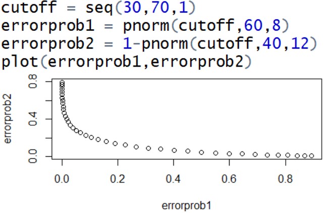
I also wonder whether I should have asked students to produce a graph of one error probability versus the other for many different cut-off values in the decision rule.  I have not used R with my business students, but I could have asked them to use Excel.  I have in mind something like the following R code and graph:


The issue of trade-offs also arises with other introductory statistics topics. My students learned about confidence intervals recently.  Here’s a favorite question of mine: Higher confidence is better than lower confidence, right?  So, why do we not always use 99.99% confidence intervals? 

The answer is that higher confidence levels produce wider confidence intervals.  Higher confidence is good, but wider intervals are bad.  In other words, there’s a trade-off between two desirable properties: high confidence and narrow intervals.

With a confidence interval for a population proportion, how many times wider is a 99.99% confidence interval than a 95% confidence interval?  The critical values are z* = 1.960 for 95% confidence, z* = 3.891 for 99.99% confidence.  This means that a 99.99% confidence interval is 3.891 / 1.960 ≈ 1.985 times wider than a 95% confidence interval.

How can a researcher achieve the best of both worlds – high confidence and a narrow interval?  The only way to achieve both is to use a very large sample size.  What are some trade-offs associated with a very large sample size?  Selecting a very large sample requires much more time, effort, and expense.  Also, increasing the sample size come with diminishing returns: You must quadruple the sample size in order to cut the interval’s width in half.


I’m tempted, but have never dared, to ask students to write an essay about how they have assessed trade-offs when making a decision of their own.  The COVID-19 crisis, which we are all trying to navigate as best we can, involves many, many trade-offs.  My students had to weigh trade-offs in deciding whether to live on campus this term, and they’ll have to do so again as they decide where to live next term.  They may have to evaluate trade-offs in deciding whether to go to their grandparents’ house for Thanksgiving dinner.  If those topics are too personal, they could also write about much less serious trade-offs, perhaps about their strategy for playing a board or card game, or deciding whether to have a salad or a cheeseburger for lunch. I could also invite students to write about trade-offs from another’s perspective, such as a mayor deciding whether to open or close schools during the COVID-19 crisis, or whether a football coach should “go for it” on fourth down*.

* This article (here) describes how analytics has led some football coaches to revise their conservative strategy on this question.


As you know, I was distracted by watching a golf tournament as I began writing this blog post.  While I was watching golf, I was also thinking about trade-offs.  Golfers have long debated whether it’s better to strive for distance or accuracy as the more important goal.  The trade-off is that you can hit the ball farther if you’re willing to sacrifice some accuracy.  On one hand, hitting the ball farther means that you’ll hit your next shot from closer to the hole.  But by giving up some accuracy, you’ll more often have to hit your next shot from the rough rather than from the fairway, so you’ll have less ability to control where your next shot goes.  On the other hand, prioritizing accuracy means achieving less distance.  With more accurate shots, you’ll more often hit your next shot from the smooth fairway where you can control your next shot better, but you’ll be farther from the hole and therefore diminish your chance to hit the next shot close.  Much of golf strategy involves navigating this trade-off.  The recent push toward analytics in sports has extended to golf, where statisticians gather and analyze lots of data to help players make decisions*.

* This article (here) from last week by golf writer Alan Shipnuck summarizes some of these developments.

And now, if you will excuse me, since the golf tournament is over and I have (ever-so-nearly) finished writing this blog post, I need to check on how my fantasy football team, the Domestic Shorthairs, is doing this week.

#71 An SBI quiz

During this past week, I introduced my students to simulation-based inference (SBI), as described in post #12, here.  I gave a follow-up quiz in our learning management system Canvas to assess how well they could apply what they learned to a study that they had not yet seen.  I give three of these application quizzes in a typical week, along with three quizzes that assess how well they followed the handout that we worked through*.  All of these quizzes consist of five questions that are auto-graded in Canvas.  I regard these quizzes as formative rather than summative, and I encourage students to help each other on the quizzes.

* Students could work through the handouts completely on their own, but most students either attend a live zoom session, during which I lead them through the handout, or watch videos that I prepare for each handout**. 

** For those of you who read about my ludicrous, comedy-of-errors experience with recording my first video (post #63, here), I am happy to report that I have recorded 83 more videos for my students since then.  Not many have gone smoothly, but all have gone much more smoothly than my first feeble attempts.

Writing auto-graded quizzes is a new experience for me.  For this blog post, I will present my auto-graded SBI quiz questions, describe my thinking behind each question, and discuss common student errors.  I will also discuss some questions that I did not ask, and I may very well second-guess some of my choices.  The quiz questions appear below in italics.


For the context in this quiz, I use a study that I described in an exam question presented in post #22, here.

Researchers presented young children (aged 5 to 8 years) with a choice between two toy characters who were offering stickers.  One character was described as mean, and the other was described as nice.  The mean character offered two stickers, and the nice character offered one sticker.  Researchers wanted to investigate whether children would tend to select the nice character over the mean character, despite receiving fewer stickers.  They found that 16 of the 20 children in the study selected the nice character.

1. What values would you enter for the inputs of a coin-tossing simulation analysis of this study?

  • Probability of heads
  • Number of tosses
  • Number of repetitions

I used the matching format in Canvas for this question.  The options presented for each of the three sub-parts were: 0.5, 0.8, 1, 10, 16, 20, and 10,000.  The correct answers are 0.5, 20, and 10,000, respectively.

As the sample proportion of children who selected the nice character, the value 0.8 makes a good option for the probability of heads.  Some students believe that the simulation is conducted with the sample value rather than the null-hypothesized value.  I chose the value 16 as a good distractor for the number of tosses, because it is the number of children in the sample who selected the nice character.  I threw in the values 1 and 10 for good measure.


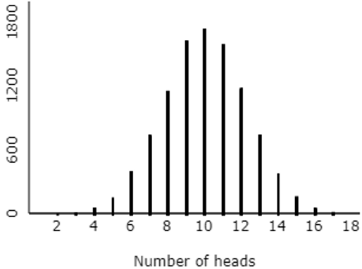
2. Consider the following graph of simulation results:

Based on this graph, which of the following is closest to the p-value?

The options presented were: 0.005, 0.100, 0.500, 0.800.  I had to keep these options pretty far apart, because we cannot determine the p-value very precisely from the graph.

Students are to realize that the p-value is approximated by determining the proportion of repetitions that produced 16 or more heads.  Although we cannot approximate the p-value very accurately from this graph, we can see that obtaining 16 or more heads did not happen very often.  The closest option is 0.005.

I considered asking students to use an applet (here) to conduct a simulation analysis for themselves and report the approximate p-value.  But I wanted this question to focus on whether they could read a graph of simulation results correctly.

I also thought about asking students to indicate how to determine an approximate p-value from the graph of simulation results.  The correct answer would have been: count the number of repetitions that produce 16 or more heads, and then divide by the number of repetitions.  Some obvious incorrect options could have been to count the repetitions that produced 10 or more heads, or to count the number of repetitions that produced exactly 10 heads.  Perhaps that would have been better than the version I asked.  I am a bit concerned that some students might have answered my question correctly simply be selecting the smallest option presented for the p-value.  On the other hand, one of the two examples presented in the handout led to a large p-value close to 0.5, so I hope my students do not necessarily think that the smallest p-value will always be the correct answer.


3. Based on this simulation analysis, do the data from this study provide strong evidence that children have a genuine preference for the nice character with one sticker rather than the mean character with two stickers?  Why?

The options presented were:

  • Yes, because it is very unusual to obtain 16 or more heads
  • Yes, because the distribution follows a bell-shaped curve
  • Yes, because the distribution is centered around 10
  • No, because it is very unusual to obtain 16 or more heads
  • No, because the distribution follows a bell-shaped curve
  • No, because the distribution is centered around 10

I like this one.  This question directly addresses the reasoning process of simulation-based inference.   The correct answer is the first one listed here.  I think the distractors are fairly tempting, because some students focus on the shape or center of the distribution, rather than thinking about where the observed result falls in the distribution.  Those misconceptions are common and important to address.

You could fault me, I suppose, for not adding if the children actually had no preference after it is very unusual to obtain 16 or more heads to the end of the correct answer.  But I think omitting that from all of the options kept the question reasonable.  In hindsight perhaps I should have written the correct answer as: Yes, because the simulation rarely produced 16 or more heads.


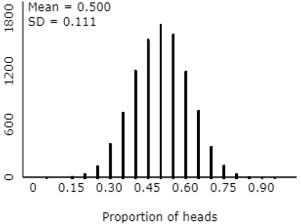
4. The following graph pertains to the same simulation results, this time displaying the distribution of the proportion of heads:

Calculate the z-score for the sample proportion of children in the study who selected the nice character with one sticker.  Report your answer with one decimal place of accuracy.

This question calls for a numerical answer rather than multiple-choice.  The correct answer is: z = (.800 – .500) / .111 ≈ 2.7*.  I allowed an error tolerance of 0.05 for the auto-grading process, so as not to penalize students who ignored my direction to use one decimal place of accuracy in their answer.

* My students have not yet studied the general expression for the standard deviation of the sampling distribution of a sample proportion, so their only option is to use the standard deviation of the 10,000 simulated sample proportions, as report in the output.

This z-score calculation is not directly related to simulation-based inference, I suppose.  But I think z-scores are worth emphasizing*, and this also foreshadows the one-proportion z-test to come.

* See post #8, End of the alphabet, here.


5. Suppose that the study had found that 13 of 20 children selected the nice character with one sticker.  How would the p-value have changed, as compared to the actual result that 16 of 20 children selected that character?

The options presented here were: larger, smaller, no change.  The correct answer is larger*, because the p-value would entail repetitions that produced 13 or more heads, which will certainly be more than those that produced 16 or more heads.

* You may have noticed that I have always presented the correct answer first in this post, but Canvas shuffled the options for my students, so different students saw different orderings.

I considered asking how the strength of evidence would change, rather than how the p-value would change.  It’s certainly possible for a student to answer the p-value question correctly, without making the connection to strength of evidence.  But it’s also possible that a student could correctly answer about strength of evidence without thinking through what that means for the p-value.  In hindsight, I wish that I had asked both versions in one question, like this:

Suppose that the study had found that 13 of 20 children selected the nice character with one sticker.  How would the p-value have changed, as compared to the actual result that 16 of 20 children selected that character, and how would the strength of evidence that children genuinely prefer the nice character have changed?  [Options: larger p-value, stronger evidence; larger p-value, weaker evidence; smaller p-value, stronger evidence; smaller p-value, weaker evidence]


As I mentioned earlier, I confine myself to asking five questions on every quiz.  I like this consistency, and I hope students appreciate that too.  But I feel no such constraint with blog posts, so now I will present five other questions that I could have asked on this quiz, all based on the same study about children selecting toy characters.

6. What are the observational units and variable in this study?  I ask these questions very often in class*, and I also ask them fairly often on assessments.  This might have worked well in matching format, with options such as: children, toy characters, which character a child selected, number of children who selected nice character, proportion of children who selected nice character.

* See post #11, Repeat after me, here.

7. Which of the following describes the null model/hypothesis?  Options could have included:

  • that children have no genuine preference between these two characters,
  • that infants genuinely prefer the nice character with one sticker to the mean character with two stickers,
  • that 80% of all infants prefer the nice character with one sticker.

8. Which of the following graphs is based on a correct simulation analysis?

9. What does the p-value represent in this study?  Options could have included:

  • the probability that 16 or more children would have selected the nice character, if in fact children have no genuine preference between the two characters
  • the probability that 10 children would have selected the nice character, if in fact children have no genuine preference between the two characters
  • the probability that 10 children would have selected the nice character, if in fact children have a genuine preference for the nice character
  • the probability that children have no genuine preference between the two characters

10. How would the p-value change if the study had involved twice as many children, and the same proportion had selected the nice character with one sticker?  The options would be: smaller, larger, no change. Students would have needed to use the applet on this question, or else relied on their intuition, because we had not yet investigated the effect of sample size on p-value or strength of evidence.

The correct answers for these additional questions are: 6. children, which character a child selected; 7. no genuine preference; 8. the graph on the right, centered at 10 with a normal-ish shape; 9. the first option presented here; 10. smaller.


Confining myself to auto-graded questions on quizzes* is a new experience that requires considerable re-thinking of my assessment questions and strategies.  In this post I have given an example of one such quiz, on the topic of simulation-based inference.  I have also tried to provide some insights into my thought process behind these questions and the various answer options for multiple-choice ones.  I have also indicated some places where I think in hindsight that I could have asked better questions.

* Not all aspects of my students’ work are auto-graded.  I assign occasional investigation assignments, like the batch testing investigation that I wrote about in my previous blog post here, for which I provide a detailed rubric to a student grader.  On exams, I use a mix of auto-graded and open-ended questions that I grade myself, as I discussed in this post #66, First step of grading exams, here.

P.S. The study about children’s toy character selections can be found here.

#70 Batch testing, part 2

I recently asked my students to analyze expected values with batch testing for a disease, which I discussed in some detail in post #39, here.  Rethinking this scenario led me to ask some new questions that I had not asked in that earlier post.

I will first re-introduce this situation, present the basic questions and analysis that my students worked through, and then ask the key question that I wish I had asked previously.  If you’d like to skip directly to the new part, scroll down to the next occurrence of “key question.” As always, questions that I pose to students appear in italics.


Suppose that 12 people need to be given a blood test for a certain disease.  Assume that each person has a 10% chance of having the disease, independently from person to person.  Consider two different plans for conducting the tests:

  • Plan A: Give an individual blood test to each person.
  • Plan B: Combine blood samples from all 12 people into one batch; test that batch.
    • If at least one person has the disease, then the batch test result will be positive, and then all 12 people will need to be tested individually.
    • If nobody has the disease, then the batch test result will be negative, and no additional tests will be needed.

Let the random variable X represent the total number of tests needed with plan B (batch testing).

a) Determine the probability distribution of X. [Hint: List the possible values of X and their probabilities.]

Even with the hint, some of my students were confused about where to begin, so I tried to guide them through the implications of the two sub-bullets describing how batch testing works.

The possible values of X are 1 (if nobody has the disease) and 13 (if at least one person has the disease).  The probabilities are: Pr(X = 1) = Pr(nobody has the disease) = (.9)12 ≈ 0.2824 by the multiplication rule for independent events, and Pr(X = 13) = 1 – Pr(nobody has the disease) = 1 – (.9)12 ≈ 0.7176.  This probability distribution can be represented in the following table:

b) If you implement plan B once, what is the probability that the number of tests needed will be smaller than it would be with plan A?

This question really stumps some students.  Because plan A always requires 12 tests, the answer is simply: Pr(X < 12) ≈ 0.2824.  My goal is for students to realize that batch testing reduces the required number of tests only about one-fourth of the time, so this criterion does not reveal any advantage of batch testing.  Maybe I need to ask the question differently, or ask a different question altogether, to direct students’ attention to this point.

c) Determine the expected value of X.

This calculation is straightforward: E(X) = 1(.9)12 + 13(1 – .912) ≈ 9.61.

d) Interpret what this expected value means in this context.

My students quickly realize that I want them to focus on long-run average when they interpret expected value (see post #18, here).  But a challenging aspect of this is to describe what would be repeated a large number of times.  In this case: If the batch testing plan were applied for a very large number of groups of 12 people, then the long-run average number of tests needed would be very close to 9.61 tests.

e) Which plan – A or B – requires fewer tests, on average, in the long run?

Maybe I should have asked this differently, perhaps in terms of choosing between plan A and plan B.  The answer is that plan B is better in the long run, because it will require about 9.61 tests on average, compared to 12 tests with plan A.


Now consider a third plan:

  • Plan C: Randomly divide the 12 people into two groups of 6 people each.  Within each group, combine blood samples from the 6 people into one batch.  Test both batches.
    • As before, a batch will test positive only if at least one person in the group has the disease.
      • Any batch that tests positive requires individual testing for the 6 people in that group.
    • As before, a batch will test negative if nobody in the group has the disease. 
      • Any batch that tests negative requires no additional testing.

Let the random variable Y represent the total number of tests needed with plan C (batch testing on two sub-groups).

f) Determine the probability distribution of Y.

Analyzing plan C is more challenging than plan B, because there are more uncertainties involved.  I advise my students to start with the best-case scenario, proceed to the worst-case, and finally tackle the remaining case. The best case is that only 2 tests are needed, because nobody has the disease. The worst case is that 14 tests are needed (the original 2 batch tests plus 12 individual tests), because at least one person in each sub-group has the disease. The remaining case is that 8 tests are needed, because at least one person in one sub-group has the disease and nobody in the other sub-group has the disease.

The most straightforward probability to determine is Pr(Y = 2), because this is the probability that none of the 12 people have the disease.  This equals (.9)12 ≈ 0.2824, just as before.

The second easiest probability to calculate is Pr(Y = 14), which is the probability that both sub-groups have at least one person with the disease.  This probability is [1 – (.9)6] for each sub-group.  The assumption of independence gives that Pr(Y =14) = [1 – (.9)6]2 ≈ 0.2195.

At this point we could simply determine Pr(Y = 8) = 1 – Pr(Y = 2) – Pr(Y = 14) ≈ .4980.  But I encouraged my students to try to calculate Pr(Y = 8) directly and then confirm that the three probabilities sum to 1, as a way to check their work.  To do this, we recognize that Y = 8 when one of the sub-groups has nobody with the disease and the other sub-group has at least one person with the disease.  A common error is for students to neglect that there are two ways for this to happen, because either sub-group could be the one that is disease-free.  This gives: Pr(Y = 8) = 2 × [1 – (.9)6] × (.9)6 ≈ .4980.

The probability distribution of Y can therefore be represented in this table:

g) Determine the expected value of Y.

This calculation is straightforward: E(Y) = 2(.2824) + 8(.4980) + 14(.2195) ≈ 7.62 tests.

h) Write a sentence or two summarizing your findings, with regard to an optimal plan for minimizing how many tests will be needed in the long run.

Students who correctly determined the expected values realize that the best of these three plans is Plan C.  If this procedure is applied for a very large number of groups, then Plan C will result in an average of about 7.62 tests per group of 12 people.  This is smaller than the average number of tests needed with Plan B (9.61) or Plan A (12.00).


Now comes the key question that I did not address in my earlier post about batch testing: Can we do even better (in terms of minimizing the average number of tests needed in the long run) than using 2 sub-groups of 6 people?  I chose the number 12 here on purpose, because it lends itself to several more possibilities: 3 sub-groups of 4, four sub-groups of 3, and six sub-groups of 2.

We can imagine groans emanating from our students at this prospect.  But we can deliver them some good news: We do not need to determine the probability distributions for the number of tests in all of these situations.  We can save ourselves a lot of bother by solving one general case and then using properties of expected values.

i) Let W represent the number of tests needed when an arbitrary number of people (n) are to be tested in a batch.  Determine the probability distribution of W and expected value of W, as a function of n.

The possible values are simply 1 and (n + 1).  We can calculate Pr(W = 1) = Pr(nobody has the disease) = .9n.  Similarly, Pr(W = n + 1) = Pr(at least one person has the disease) = 1 – .9n.  The expected value is therefore: E(W) = (1 × .9n) + (n + 1) × (1 – .9n) = n + 1 – n(.9n).  This holds when n ≥ 2.

j) Confirm that this general expression gives the correct expected value for n = 12 people.

I encourage my students to look for ways to check their work throughout a complicated process. Plugging in n = 12 gives: E(W) = 12 + 1 – 12(.912) ≈ 9.61 tests. Happily, this is the same value that we determined earlier.

k) Use the general expression to determine the expected value of the number of tests with a batch of n = 6 people. 

This gives: E(W) = 6 + 1 – 6(.96) ≈ 3.81 tests

l) How does this compare to the expected value for plan C (dividing the group of 12 people into two sub-groups of 6) above?  Explain why this makes sense.

This question holds the key to our short-cut. This expected value of 3.81 is equal to one-half of the expected number of tests with plan C, which was 7.62 tests.  This is not a fluke, because we can express Y (the total number of tests with two sub-groups of 6) as Y = Y1 + Y2, where Y1 is the number of tests with the first sub-group of 6 people, and Y2 is the number of tests with the second sub-group of 6 people.  Properties of expected value then establish that E(Y1 + Y2) = E(Y1) + E(Y2).

This same idea will work, and save us considerable time and effort, for all of the other sub-group possibilities that we mentioned earlier.

m) Determine the expected value of the number of tests for three additional plans: three sub-groups of 4 people each, four sub-groups of 3 people each, and six sub-groups of 2 people each.  [Hint: Use the general expression and properties of expected value.]

With a sub-group of 4 people, the expected number of tests with one sub-group is: 4 + 1 – 4(.94) ≈ 2.3756.  The expected value of the number of tests with three sub-groups of 4 people is therefore: 3(2.3756) ≈ 7.13 tests.

With a sub-group of 3 people, the expected number of tests with one sub-group is: 3 + 1 – 3(.93) ≈ 1.813.  The expected value of the number of tests with four sub-groups of 3 people is therefore: 4(1.813) ≈ 7.25 tests.

With a sub-group of 2 people, the expected number of tests with one sub-group is: 2 + 1 – 2(.92) = 1.38.  The expected value of the number of tests with six sub-groups of 2 people is therefore: 6(1.38) = 8.28 tests.

n) Write a paragraph to summarize your findings about the optimal sub-group composition for batch-testing in this situation.

The following table summarizes our findings about expected values:

With a group of 12 people, assuming independence and a disease probability of 0.1 per person, the optimal sub-group composition is to have 3 sub-groups of size 4 people each.  This produces an expected value of 7.13 for the number of tests to be performed.  This is 39.6% fewer tests than the 12 that would have to be conducted without batch testing.  This is also 24.5% fewer tests than would be performed with just one batch.  (See post #28, here, for my pet peeve about misconceptions involving percentage differences.)


Let’s conclude with two more extensions of this batch testing problem:

o) How do you predict the optimal sub-group composition to change with a smaller probability that an individual has the disease?  Change the probability to 0.05 and re-calculate the expected values to test your prediction.

It makes sense that larger sub-groups would be more efficient with a more rare disease.  With p = 0.05, we obtain the following expected values for the total number of tests:

In this case with a more rare disease (p = 0.05), the optimal strategy is to divide the 12 people into two groups of 6 people each.  This results in 5.18 tests on average in the long run.

p) How would the optimal sub-group composition change (if at all) if there were twice as many people (24) in the group?

We can simply double the expected values above.  We also have new possibilities to consider: three sub-groups of size 8, and two sub-groups of size 12.  For the p = 0.05 case, this produces the same optimal sub-group size as before, 6 people per sub-group, as shown in the following table of  expected values:


Batch testing provides a highly relevant application of expected values for discrete random variables that can also help students to develop problem-solving skills. Speaking of relevance, you may have noticed that COVID-19 and coronavirus did not appear in this post until now.  I did not want to belabor this connection with my students, but I trust that they could not help but recognize the potential applicability of this technique to our current challenges.  I also pointed my students to an interactive feature from the New York Times here, an article in the New York Times here, and an article in Significance magazine here.

P.S. I recorded a video presentation of this batch testing for the College Board, which you can find here.