I often tell my students that I make mistakes in class on purpose as a teaching strategy, to encourage them to pay close attention, check my work regularly rather than simply copy what I say into their notes, and speak up when they notice something that they question.
This is partially true, but most of the mistakes that I make in class are, of course, genuine ones rather than purposeful. I admit that I sometimes try to bluff my way through, with tongue firmly planted in cheek, claiming that my mistake had been intentional, an application of that teaching strategy.
Thanks very much to the careful blog reader who spotted a mistake of mine in today’s post. In a follow-up discussion to the first example, I wrote: If the marginal percentages had been 28% and 43%, then the largest possible value for the intersection percentage would have been 28% + 43% = 71%. This is not true, because the intersection percentage can never exceed either of the marginal percentages. With marginal percentages of 28% and 43%, the largest possible value for the intersection percentage would be 28%.
Perhaps I was thinking of the largest possible percentage for the union of the two events, which would indeed be 28% + 43% = 71%. Or perhaps I was not thinking much at all when I wrote that sentence. Or perhaps, just possibly, you might be so kind as to entertain the notion that I made this mistake on purpose, as an example of a teaching strategy, which I am now drawing to your attention?
My students and I have spent the last three weeks studying probability*. At the end of Friday’s class session, one of the students asked a great question. Paraphrasing a bit, she asked: We can answer some of these questions by thinking rather than calculating, right? I was delighted by her question and immediately replied: Yes, absolutely! I elaborated that some questions call for calculations, so it’s important to know how to use probability rules and tools. Those questions usually require some thinking as well as calculating. But other questions ask you to think things through without performing calculations. Let me show you some of the questions that I have asked in this unit on probability**.
* This course is the first of a two-course introductory sequence for business students.
** Kevin Ross’s guest post (#54, here) provided many examples of probability questions that do not require calculations.
My students saw the following questions on a quiz near the beginning of the probability unit:
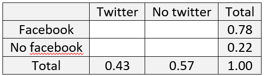
1. Suppose that 78% of the students at a particular college have a Facebook account and 43% have a Twitter account.
a) Using only this information, what is the largest possible value for the percentage who have both a Facebook account and a Twitter account? Describe the (unrealistic) situation in which this occurs.
b) Using only this information, what is the smallest possible value for the percentage who have both a Facebook account and a Twitter account? Describe the (unrealistic) situation in which this occurs.
Even though these questions call for a numerical response, and can therefore be auto-graded, they mostly require thinking rather than plugging into a rule. We had worked through a similar example in class, in which I encouraged students to set up a probability table to think through such questions. The marginal probabilities given here produce the following table:
For part (a), students need to realize that the percentage of students with both kinds of accounts cannot be larger than the percentage with either account individually. The largest possible value for that intersection probability is therefore 0.43, so at most 43% of students could have had both kinds of accounts. If this were not an auto-graded quiz, I would have also asked for a description of this (unrealistic) scenario: that every student with a Twitter account also has a Facebook account.
Part (b) is more challenging. A reasonable first thought is that the smallest possible probability could be 0. But then Pr(Facebook or Twitter) would equal 0.78 + 0.43, and 1.21 is certainly not a legitimate probability. That calculation points to the correct answer: Because Pr(Facebook or Twitter) cannot exceed 1, the smallest possible value for Pr(Facebook or Twitter) is 1.21 – 1 = 0.21. At least 21% of students must have both kinds of accounts. This unrealistic scenario requires that every student have a Facebook account or a Twitter account.
Notice that if the two given probabilities had not added up to more than 1, then the smallest possible value for the intersection probability would have been 0%.
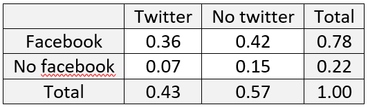
The remaining three parts of the quiz provided students with a specific value (36%) for the percentage of students with both a Facebook and Twitter account and then asked for routine calculations:
c) What percentage of students have at least one of these accounts?
d) What percentage of students have neither of these accounts?
e) What percentage of students have one of these accounts but not both?
These percentages turn out to be 85%, 15%, and 49%, respectively. The easiest way to determine these is to complete the probability table begun above:
The following questions appear on a practice exam that I gave my students to prepare for this coming Friday’s exam:
2. Suppose that a Cal Poly student is selected at random. Define the events E = {randomly selected student is an Engineering major} and T = {randomly selected student is taking STAT 321 this term}. For each of the following pairs of probabilities, indicate which probability is larger, or if the two probabilities are the same value. You might want to consider the following information: A few thousand students at Cal Poly are Engineering majors. A few dozen students are taking STAT 321 this term. Less than a handful of current STAT 321 students are not Engineering majors.
a) Pr(E), Pr(T)
b) Pr(E), Pr(E and T)
c) Pr(T), Pr(E or T)
d) Pr(E), Pr(E | T)
e) Pr(T | E), Pr(E | T)
These question requires only thinking, no calculations. I purposefully avoided giving specific numbers at the end of this question.
Part (a) is an easy one, because there a lot more Engineering majors than there are STAT 321 students. For part (b), students are to realize that (E and T) is a subset of E, so Pr(E) must be larger than Pr(E and T). Similarly in part (c), T is a subset of (E or T), so Pr(E or T) must be larger than Pr(T). For part (d), most STAT 321 students are Engineering majors, so Pr(E | T) is larger than Pr(E). Finally, relatively few Engineering majors take STAT 321 in any one term, so Pr(E | T) is also larger than Pr(T | E).
My students completed a fairly long assignment that asked them to apply the multiplication rule for independent events to calculate various probabilities that a system functions successfully, depending on whether components are connected in series (which requires all components to function successfully) or in parallel (which requires at least one component to function successfully). The final two parts of this assignment were:
3. Suppose that three components are connected in a system. Two of the components form a sub-system that is connected in parallel, which means that at least one of these two components must function successfully in order for the sub-system to function successfully. This sub-system is connected in series with the third component, which means that both the sub-system and the third component must function successfully in order for the entire system to function successfully. Suppose that the three components function independently and that the probabilities of functioning successfully for the three components are 0.7, 0.8, and 0.9. Your goal is to connect the system to maximize the probability that the system functions successfully.
i) Which two components would you select to form the sub-system, and which would you select to be connected in series with the sub-system? Explain your choice.
j) Determine the probability that the system functions successfully with your choice. Justify the steps of your calculation with the appropriate probability rules.
The first of these questions can be answered without performing calculations. Because the component connected in series must function successfully in order for the system to function successfully, that component should be the most reliable one: the one with probability 0.9 of functioning successfully. The remaining two components, with success probabilities 0.8 and 0.7, should be connected in parallel.
The calculation for part (j) certainly does require applying probability rules correctly. The probability that this system functions successfully can be written as*: Pr[(C7 or C8) and C9]. The multiplication rule for independent events allows us to write this as: Pr(C7 or C8) × Pr(C9). Applying the addition rule on the first term gives: [Pr(C7) + Pr(C8) – Pr(C7 and C8)] × Pr(C9). Then one more application of the multiplication rule gives: [Pr(C7) + Pr(C8) – Pr(C7) × Pr(C8)] × Pr(C9). Plugging in the probability values gives: [0.7 + 0.8 – 0.7×0.8] × 0.9, which is 0.846.
* I’m hoping that my notation here will be clear without my having to define it. I consider this laxness on my part a perk of blog writing as opposed to more formal writing.
Notice that a student could have avoided thinking through the answer to (i) by proceeding directly to (j) and calculating probabilities for all possible arrangements of the components. I do not condone that strategy, but I do encourage students to answer probability questions in multiple ways to check their work. The other two probabilities (for the system functioning successfully) turn out to be 0.776 if the 0.8 probability component is connected in series and 0.686 if the 0.7 probability component is connected in series.
Finally, here’s the in-class example that prompted my student’s question at the top of this blog post:
4. Suppose that Zane has a 20% chance of earning a score of 0 and an 80% chance of earning a score of 5 when he takes a quiz. Suppose also that Zane must choose between two options for calculating an overall quiz score: Option A is to take one quiz and multiply the score by 10, Option B is to take ten (independent) quizzes and add their scores.
a) Which option would you encourage Zane to take? Explain.
b) Which option do you suspect has a larger expected value, or do you suspect that the expected values will be the same?
c) Use properties of expected value to determine the expected value of his overall score with each option. Comment on how they compare.
d) Which option do you suspect has a larger standard deviation, or do you suspect that the standard deviations will be the same?
e) Use properties of variance to determine the standard deviation of his overall score with each option. Comment on how they compare.
f) If Zane’s goal is to maximize his probability of obtaining an overall score of 50 points, which option should he select? Explain.
g) Calculate the probability, for each option, that Zane scores 50 points. Comment on how they compare.
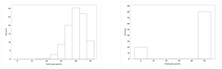
h) The following graphs display the probability distributions of Zane’s overall quiz score with these two options. Which graph goes with which option? Explain.
The key idea here is that multiplying a single quiz score by 10 is a much riskier, all-or-nothing proposition than adding scores for 10 independent quizzes. A secondary goal is for students to learn how to apply rules of expected values and variances to multiples and sums of random variables.
The expected value of Zane’s score on a single quiz is 4.0, and the standard deviation of his score on a single quiz is 2.0. The expected value of the random variable (10×Z) is the same as for the random variable (Z1 + Z2 + … + Z10), namely 40.0 quiz points. This means that neither option is better for Zane in terms of long-run average.
But this certainly does not mean that the two options yield identical distributions of results. The variance of (10×Z) is 102 × 4.0 = 400, so the standard deviation is 20.0. The variance for (Z1 + Z2 + … + Z10) is much smaller: 10 × 4.0 = 40, so the standard deviation is approximately 6.325.
Zane has an 80% chance of obtaining an overall quiz score of 50 with option A, because he simply needs to score a 5 on one quiz. With option B, he only achieves a perfect overall score of 50 if he earns a 5 on all 10 quizzes, which has probability (0.8)10 ≈ 0.107.
The graph on the left above shows the probability distribution for option B, and the graph on the right corresponds to option A. The graphs reveal the key idea that option A is all-or-nothing, while option B provides more consistency in Zane’s overall quiz score.
The great mathematician Laplace reportedly said that “probability theory is nothing but common sense reduced to calculations.” I wish I had thought quickly enough on my feet to mention this in response to my student’s comment in class on Friday. I’ll have to settle for hoping that my probability questions lead students to develop a habit of mind to think clearly and carefully about randomness and uncertainty, along with the ability to perform probability calculations.
I told my students at the beginning of our last class session that I was especially excited about class that day for several reasons:
It was a Friday.
We were about to work through our thirteenth handout of the term, a lucky number.
The date was October 16, the median day for the month of October.
We had reached the end of week 5 of our 10-week quarter, the halfway point.
The topic for the day was my favorite probability rule, in fact my favorite mathematical theorem: Bayes’ rule.
The first two examples that we worked through concerned twitter use and HIV testing, as described in post #10, My favorite theorem, here.
The third and final example of the day presented this scenario: Suppose that Jasmine* has a 70%** chance of knowing (with absolute certainty) the answer to a randomly selected question on a multiple-choice exam. When she does not know the answer, she guesses randomly among the five options.
* I had always used the name Brad with this made-up example. But I realized that I had used an example earlier in the week with the names Allan, Beth, Chuck, Donna, and Ellen, so I thought that I should introduce a bit of diversity into the names of fictional people in my made-up probability examples. I did a google search for “popular African-American names” and selected Jasmine from the list that appeared.
** When I first rewrote this example with Jasmine in place of Brad, my first thought was to make Jasmine a stronger student than Brad, so I wrote that she has an 80% rather than a 70% chance of knowing the answer for sure. Later I realized that this change meant that the value 20% was being used for the probability of her guessing and also for the probability of her answering correctly given that she is guessing. I wanted to avoid this potential confusion, so I changed back to a 70% chance of Jasmine knowing the answer.
a) Before we determine the solution, make a prediction for the probability that Jasmine answers a randomly selected question correctly. In other words, make a guess for the long-run proportion of questions that she would answer correctly.
I hope students realize that this probability should be a bit larger than 0.7. I want them to reason that she’s going to answer 70% correctly based on her certain knowledge, and she’s also going to answer some correctly when she’s guessing just from blind luck. I certainly do not expect students to guess the right answer, but it’s not inconceivable that some could reason that she’ll answer correctly on 20% of the 30% that she guesses on, which is another 6% in addition to the 70% that she knows for sure, so her overall probability of answering correctly is 0.76.
Next I ask students to solve this with a table of counts for a hypothetical population, just as we did for the previous two examples (again see post #10, here). This time I only provide them with the outline of the table rather than giving row and column labels. b) Fill in the row and column labels for the table below:
To figure out what labels to put on the rows and columns, I remind students that the observational units here are 100 multiple choice questions, and they need to think about the two variables that we record about each question. It takes most students a little while to realize that the two variables are: 1) whether Jasmine knows the answer or guesses, and 2) whether Jasmine answers the question correctly or not. This leads to:
c)Fill in the table of counts for a hypothetical population of 100 questions. We proceed through the following calculations:
Jasmine will know the answer for 70% of the 100 questions, which is 70.
She will guess at the answer for 100 – 70 = 30 questions.
For the 70 questions where she knows the answer, she will correctly answer all 70, leaving 0 that she will answer incorrectly.
For the 30 questions on which she guesses, we expect her to answer correctly on one-fifth of them, which is 6.
That leaves 30 – 6 = 24 questions for which she will guess and answer incorrectly.
The column totals are therefore 76 correctly answered questions and 24 incorrect.
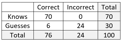
The completed table is shown here:
d) Use the table to report the probability that Jasmine answers a randomly selected question correctly. This can read from the table to be: Pr(correct) = 76/100 = 0.76.
e) Show how this unconditional probability (of answering a randomly selected question correctly) can be calculated directly as a weighted average of two conditional probabilities. This is more challenging for students, but I think the idea of weighted average is an important one. I want them to realize that the two conditional probabilities are: Pr(correct | know) = 1.0 and Pr(correct | guess) = 0.2. The weights attached to these are the probabilities of knowing and of guessing in the first place: Pr(know) = 0.7 and Pr(guess) = 0.3. The unconditional probability of answering correctly can be expressed as the weighted average 0.7×1.0 + 0.3×0.2 = 0.76.
f) Determine the conditional probability, given that Jasmine answers a question correctly, that she actually knows the answer. Some students think at first that this conditional probability should equal one, but they realize their error when they are asked whether it’s possible to answer correctly even when guessing. Returning to the table, this conditional probability is calculated to be: 70/76 ≈ 0.921.
g) Interpret this conditional probability in a sentence. Jasmine actually knows the answer to about 92.1% of all questions that she answers correctly in the long run.
h) Show how to calculate this conditional probability directly from Bayes’ rule. The calculation is: Pr(know | correct) = [Pr(correct | know) × Pr(know)] / [Pr(correct | know) × Pr(know) + Pr(correct | guess) × Pr(guess)] = (1×0.7) / (1×0.7 + 0.2×0.3) = 0.70 / 0.76 ≈ 0.921. I try to impress upon students that even though this calculation looks more daunting with the formula than from filling in the table, the calculations are exactly the same, as seen by our ending up with 0.70/0.76 from the formula and 70/76 from the table. I also emphasize that I think the table provides an effective and understandable way to organize the calculations.
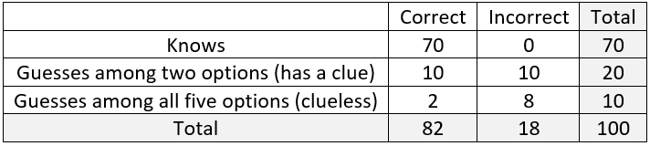
Here’s a fun extension of this example: Continue to suppose that Jasmine has a 70% chance of knowing (with absolute certainty) the answer to a randomly selected question on a multiple-choice exam. But now there’s also a 20% chance that she can eliminate three incorrect options, and then she guesses randomly between the remaining two options, one of which is correct. For the remaining 10% chance, she has no clue and so guesses randomly among all five options.
i) Before conducting the analysis, do you expect the probability that she answers a question correctly to increase, decrease, or remain the same? Explain. Then do the same for the conditional probability that she knows the answer given that she answers correctly.
Most students have correct intuition for the first of these questions: If Jasmine can eliminate some incorrect options, then her probability of answering correctly must increase. The second question is more challenging to think through: Now that she has a better chance of guessing the correct answer, the conditional probability that she knows the answer, given that she answer correctly, decreases.
j) Modify the table of hypothetical counts to determine these two probabilities. Students must first realize that the table now needs three rows to account for Jasmine’s three levels of knowledge. The completed table becomes:
The requested probabilities are: Pr(correct) = 82/100 = 0.82 and Pr(know | correct) = 70/82 ≈ 0.854. Jasmine’s ability to eliminate some incorrect options has increased her probability of answering correctly by six percentage points from 76% to 82%. But our degree of belief that she genuinely knew the answer, given that she answered correctly, has decreased by a bit more than six percentage points, from 92.1% to 85.4%.
I confess that I did not have time to ask students to work through this extension during Friday’s class. I may give it as an assignment, or as a practice question for the next exam, or perhaps as a question on the next exam itself.
I have mentioned before that I give lots and lots of quizzes in my courses (see posts #25 and 26, here and here). This is even more true in my first-ever online course. I generally assign three handout quizzes and three application quizzes per week. The handout quiz aims to motivate students to work through the handout, either by attending a live zoom session with me, or on their own, or by watching a video that I prepare for each handout. The application quiz asks students to apply some of the topics from the handout to a new situation. I also occasionally assign miscellaneous quizzes. With regard to Bayes’ rule, I have asked my students to watch a video (here) that presents the idea behind Bayes’ rule in an intuitive and visually appealing way. I wrote a miscellaneous quiz to motivate students to watch and learn from this video.
The author of this video, Grant Sanderson, argues that the main idea behind Bayes’ rule is that “evidence should not determine beliefs but update them.” I think the Jasmine example of knowing versus guessing can help students to appreciate this viewpoint. We start with a prior probability that Jasmine knows the answer to a question, and then we update that belief based on the evidence that she answers a question correctly. Do I know with absolute certainty that this example helps students to understand Bayes’ rule? Of course not, but I like the example anyway. More to the point, the evidence of my students’ reactions and performances on assessments has not persuaded me to update my belief in a pessimistic direction.
One of my favorite professional activities has been interviewing statistics teachers and statistics education researchers for the Journal of Statistics Education. I have conducted 26 such interviews for JSE over the past ten years. I have been very fortunate to chat with some of the leaders in statistics education from the past few decades, including many people who have inspired me throughout my career. I encourage you to take a look at the list and follow links (here) to read some of these interviews.
Needless to say, I have endeavored to ask good questions in these interviews. Asking interview questions is much easier than answering them, so I greatly appreciate the considerable time and thoughtfulness that my interview subjects have invested in these interviews. I hope that my questions have provided an opportunity to:
1. Illuminate the history of statistics education, both in years recent and back a few decades. A few examples:
Dick Scheaffer describes how the AP Statistics program began.
Mike Shaughnessy talks about how NCTM helped to make statistics more prominent in K-12 education.
Chris Franklin and Joan Garfield discuss how ASA developed its GAISE recommendations for K-12 and introductory college courses.
Jackie Dietz describes the founding of the Journal of Statistics Education.
Dennis Pearl explains how CAUSE (Consortium for the Advancement of Undergraduate Statistics Education) came to be.
George Cobb describes his thought processes behind his highly influential writings about statistics education.
Nick Horton shares information about the process through which ASA developed guidelines for undergraduate programs in statistical science.
David Moore, Roxy Peck, Jessica Utts, Ann Watkins, and Dick De Veaux talk about how their successful textbooks for introductory statistics came about.
2. Illustrate different pathways into the field of statistics education. Many of these folks began their careers with statistics and/or teaching in mind, but others started or took a detour into engineering or physics or psychology or economics. Some even studied fields such as dance and Russian literature.
3. Indicate a variety of ways to contribute to statistics education. Some interviewees teach in high schools, others in two-year colleges. Some teach at liberal arts colleges, others in research universities. Some specialize in teaching, others in educational research. All have made important contributions to their students and colleagues.
4. Provide advice about teaching statistics and for pursuing careers in statistics education. My last question of every interview asks specifically for advice toward those just starting out in their careers. Many of my other questions throughout the interviews solicit suggestions on a wide variety of issues related to teaching statistics well.
5. Reveal fun personal touches. I have been delighted that my interviewees have shared fun personal tidbits about their lives and careers. Once again, a few examples:
George Cobb describes his experience as the victim of an attempted robbery, which ended with his parting company on good terms with his would-be assailant.
David Moore tells of losing an annual bet for 18 consecutive years, which required him to treat his friend to dinner at a restaurant of the friend’s choosing, anywhere in the world.
Ron Wasserstein shares that after he and his wife raised their nine children, they adopted two ten-year-old boys from Haiti.
Deb Nolan mentions a dramatic career change that resulted from her abandoning plans for a New Year’s Eve celebration.
Joan Garfield reveals that she wrote a memoir/cookbook and her life and love of food.
Dennis Pearl mentions a challenge that he offers to his students, which once ended with his delivering a lecture while riding a unicycle.
Chris Franklin relates that her favorite way to relax is to keep a personal scorebook at a baseball game.
Larry Lesser shares an account of his epic contest on a basketball court with Charles Barkley.
My most recent interview (here) is with Prince Afriyie, a recent Cal Poly colleague of mine who now teaches at the University of Virginia. Prince is near the beginning of his teaching career as a college professor, and his path has been remarkable. He started in Ghana, where he was inspired to study mathematics by a teacher whom he referred to as Mr. Silence. While attending college in Ghana, Prince came to the United States on a summer work program; one of his roles was a paintball target at an amusement park in New Jersey. Serendipity and initiative enabled Prince to stay in the United States to complete his education, with stops in Kentucky, Indiana, and Pennsylvania on his way to earning a doctorate in statistics. Throughout his education and now into his own career, Prince has taught and inspired students, as he was first inspired by Mr. Silence in his home country. Prince supplies many fascinating details about his inspiring journey in the interview. I also asked Prince for his perspective on the two world-changing events of 2020 – the COVID-19 pandemic and the widespread protests for racial justice.
As I mentioned earlier, I conclude every interview with a request for advice aimed at those just beginning their career in statistics education. Jessica Utts paid me a very nice compliment when she responded that teachers who read these interviews might benefit from asking themselves some of the more general questions that I ask of my interviewees. Here are some questions that I often ask, which may lead to productive self-reflection:
Which came first – your interest in statistics or your interest in education?
What were you career aspirations at age 18?
What have you not changed about your teaching of statistics over the years?
On what do you pride yourself in your teaching?
What do you regard as the most challenging topic for students to learn, and how you approach this topic?
What is your favorite course to teach, and why?
In this time of data science, are you optimistic or pessimistic about the future of statistics?
What do you predict as the next big thing in statistics education?
What advice do you offer for those just beginning their career in statistics education?
You might also think about how you would answer two fanciful questions that I often ask for fun:
If time travel were possible, and you could travel to the past or future without influencing the course of events, what point in time would you choose? Why?
If I offer to treat you and three others to dinner anywhere in the world, with the condition that the dinner conversation would focus on statistics education, whom would you invite, and where would you dine?
P.S. If you have a chance to read some of these interviews, I would appreciate hearing your feedback (here) on questions such as:
Who would you like me to interview in the near future?
What questions would you like me to ask?
Would you prefer shorter interviews?
Would you prefer to listen to interviews on a podcast?
P.P.S. For those wondering if I graded my exams last week after finally concluding the all-important procrastination step (see post #66, First step of grading exams, here): Thanks for asking, and I happily report that I did.
I gave my first exam of the term, my first online exam ever, this past Friday. As I sat down to grade my students’ responses for the first time in almost sixteen months, I realized that I had almost forgotten the crucial first step of grading exams: Procrastinate!
I have bemoaned the fact that I have so much less time available to concentrate on this blog now that I have returned to full-time teaching, as compared to last year while I was on leave. So, what better way to procrastinate from my grading task than by engaging in the much more enjoyable activity of writing a blog post?
What should I write about? That’s easy: I will tell you a bit about the exam whose grading I am neglecting at this very moment.
Students took this exam through Canvas, our learning management system*. This is a first for me, as my students in previous years took exams with paper and pencil. I included a mix of questions that were auto-graded (multiple choice and numerical answer) and free-response questions that I will grade after I finish the all-important first step of procrastinating. Roughly two-thirds of the points on the exam were auto-graded. I wrote several different versions of many questions in an effort to discourage cheating. Students had 90 minutes to complete the exam, and they were welcome to select any continuous 90-minute period of time between 7am and 7pm. Students were allowed to use their notes. Topics tested on the exam including basic ideas of designing studies and descriptive statistics.
* In post #63 (My first video, here), I referred to Canvas as a course management system. Since then I realized that I was using an antiquated term, and I have been looking for an opportunity to show that I know the preferred term is now learning management system.
Some of the questions that I asked on this exam appear below (in italics):
1. Suppose that the observational units in a study are the national parks of the United States. For each of the following, indicate whether it is a categorical variable, a numerical variable, or not a variable.
the area (in square miles) of the national park
whether or not the national park is in California
the number of national parks that are to the east of the Mississippi River
whether there are more national parks to the east of the Mississippi River than to the west of the Mississippi River
the number of people who visited the national park in September of 2020
I give my students lots of practice with this kind of question (see post #11, Repeat after me, here), but some continue to struggle with this. Especially challenging is noticing the ones that are not variables for these observational units (parts c and d). Each student saw one of four variations on this question. The observational units in the different version were patients who visited the emergency room at the local hospital last week, the commercial flights that left the San Luis Obispo airport last month, and customers at a local In-n-Out fast food restaurant on a particular day. I posed this as a “matching” question in Canvas, where each of the five parts had the same three options available.
2. Suppose that the ten players on basketball team A have an average height of 76 inches, and the ten players on basketball team B have an average height of 80 inches. Now suppose that one player leaves team A to join team B, and one player leaves team B to join team A. How would the average heights of the two teams change? The options that I presented were: No change, Both averages would increase, Both averages would decrease, The average would increase for A and decrease for B, The average would decrease for A and increase for B, It is impossible to say without more information.
The correct option is the last one: It is impossible to say without more information. My goal here was for students to understand that players’ heights vary on both teams, so we cannot state any conclusions about how the averages would change without knowing more about the heights of the individual players who changed teams.
3. San Diego State’s admission rate for Fall 2019 was 34.13%, compared to 28.42% for Cal Poly – SLO’s. Determine the percentage difference between these admission rates. In other words, San Diego State’s admission rate was higher than Cal Poly – SLO’s by ___ %. Enter your answer as a number, with two decimal places of accuracy. Do not enter the % symbol.
As I mentioned throughout post #28 (A pervasive pet peeve, here), I emphasize how a difference in proportions is not equivalent to a percentage difference. This question assessed whether students took my emphasis to heart. Each student answered one of four versions of this question, with different campuses being compared. I obtained the data on admission rates from the dashboard here.
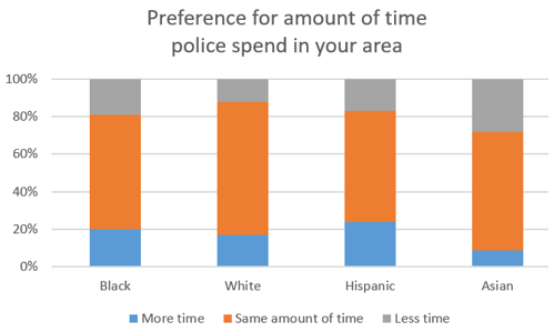
4. A series of questions referred to the following graph from a recent Gallup study (here):
The most challenging question in this series was a very basic one: How many variables are represented in this graph? The correct answer is 2, race and preference for how much time police spend in the area. The other options that I presented were 1, 3, 4, and 12.
5. Another series of questions was based on this study (available here): Researchers surveyed 120 students at Saint Lawrence University, a liberal arts college with about 2500 students in upstate New York. They asked students whether or not they have ever pulled an all-nighter (stayed up all night studying). Researchers found that students who claimed to have never pulled an all-nighter had an average GPA (grade point average) of 3.1, compared to 2.9 for students who claimed to have pulled an all-nighter. Some basic questions included identifying the type of study, explanatory variable, and response variable. These led to a question about whether a cause-and-effect conclusion can legitimately be drawn from this study, with a follow-up free-response question* asking students to explain why or why not.
* Oh dear, I just reminded myself of the grading that I still need to do. This procrastination step is fun but not entirely guilt-free.
Some other free-response questions waiting for me to grade asked students to:
6. Create a hypothetical example in which IQR = 0 and the mean is greater than the median. I think this kind of question works well on an online exam. Different students should give different responses, so I hope this question encourages independent thinking and discourages cheating. (See post #31, Create your own example, part 1, here, for many more questions of this type.)
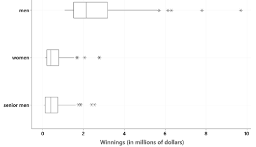
7. Write a paragraph comparing and contrasting the distribution of money winnings in 2019 on three professional golf tours – men’s, women’s, and senior men’s, as displayed in the boxplots:
I am looking for students to compare center, variability, and shape across the three distributions. They should also comment on outliers and relate their comments to the context.
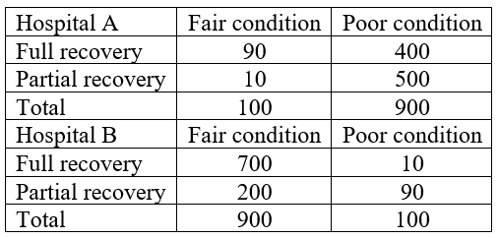
8. Describe and explain the oddity concerning which hospital performed better, in terms of patients experiencing a complete recovery, for the data shown in the following tables of counts:
I expect this to be one of the more challenging questions on the exam. Students need to calculate correct proportions, comment on the oddity that Hospital A does worse overall despite doing better for each condition, and explain that Hospital A sees most of the patients in poor condition, who are less likely to experience a full recovery than those in fair condition.
Writing my exam questions in Canvas, and preparing several versions for many questions, took considerably more time than my exam writing in the past. But of course Canvas has already saved me some time by auto-grading many of the questions. I should also be pleased that Canvas will also add up students’ scores for me, but I always enjoyed that aspect of grading, largely because it was the last part and provided a sense of completion and accomplishment.
Hmm, I probably should not be imagining an upcoming sense of completion and accomplishment while I am still happily immersed in the procrastination step of the exam-grading process. I must grudgingly accept that it’s time for me to proceed to step two. If only I could remember what the second step is …
Join 675 other subscribers
About this blog
This weekly blog provides ideas, examples, activities, assessments, and advice for teaching introductory statistics, all based on a three-word teaching philosophy: Ask good questions.
Each post aims to be both practical and thought-provoking.
See the first blog post (here) for answers to ten questions about this blog.