Skip to content

Archive for

#17 Random babies

Be forewarned that what you are about to read is highly objectionable. The topic is an introduction to basic ideas of randomness and probability, but that’s not the offensive part.  No, the despicable aspect is the context of the example, which I ask you to accept in the spirit of silliness intended.

One of the classic problems in probability is the matching problem.  When I first studied probability, this was presented in the context of a group of men at a party who throw their hats into the middle of a room and later retrieve their hats at random.  As I prepared to present this problem at the start of my teaching career, I wanted to use a context that would better capture students’ attention.  I described a hospital that returns newborn babies to their mothers at random.  Of course I realized that this context is horrific, but I thought it might be memorable, and I was hoping that it’s so far beyond the pale as to be laughable.  On the end-of-course student evaluations, one question asked what should be changed about the course, and another asked what should be retained.  For the latter question, several of my students wrote: Keep the random babies!  I have followed this advice for thirty years.

If you’d prefer to present this activity with a context that is value-neutral and perhaps even realistic, you could say that a group of people in a crowded elevator drop their cell phones, which then get jostled around so much that the people pick them up at random. That’s a value-neutral and perhaps even realistic setting. It’s also been suggested to me that the context could be a veterinarian who gives cats back to their owners at random*!

* In case you missed post #16 (here), I like cats.


After I describe this scenario to students, for the case with four babies and mothers, I ask: Use your intuition to arrange the following events in order, from least likely to most likely:

  • None of the four mothers gets the correct baby.
  • At least one of the four mothers gets the correct baby.
  • All of the four mothers gets the correct baby.

At this point I don’t care how good the students’ intuitions are, but I do want them to think about these events before we begin to investigate how likely they are.  How will we conduct this investigation?  Simulate!

Before we proceed to use technology, we start with a by-hand simulation using index cards.  I give four index cards to each student and ask them to write a baby’s first name on each card.  Then I ask students to take a sheet of scratch paper and divide it into four sections, writing a mother’s last name in each section*.  You know what comes next: Students shuffle the cards (babies) and randomly distribute them to the sections of the sheet (mothers).  I ask students to keep track of the number of mothers who get the correct baby, which we call the number of matches.  Then I point out that just doing this once does not tell us much of anything. We need to repeat simulating this random process for a large number of repetitions.  I usually ask each student to repeat this three times.

* I used to provide students with names, but I think it’s more fun to let them choose names for themselves.  I emphasize that they must know which baby goes with which mother.  I recommend that they use alliteration, for example with names such as Brian Bahmanyar and Hector Herrera and Jacob Jaffe and Sean Silva**, to help with this.

** These are the names of four graduates from the Statistics program at Cal Poly. Check out their (and others’) alumni updates to our department newsletter (here) to learn about careers that are available to those with a degree in statistics.

Once the students have completed their three repetitions, each goes to the board, where I have written the numbers 0, 1, 2, 3, 4 across the top*, and students put tally marks to indicate their number of matches for each of their repetitions.  Then we count the tallies for each possible value, and finally convert these counts to proportions.  Here are some sample results:

* I make the column for exactly 3 matches very skinny, because students should realize that it’s impossible to obtain this result (because if 3 mothers get the right baby, then the remaining baby must go to the correct mother also).

At this point I tell students that these proportions are approximate probabilities.  I add that the term probability refers to the long-run proportion of times that the event would occur, if the random process were repeated for a very large number of repetitions.  Based on the by-hand simulation with 96 repetitions shown above, our best guesses are that nobody would receive the correct baby in 40.6% of all repetitions and that all four mothers would get the correct baby in 3.1% of all repetitions.


How could we produce better approximations for these probabilities?  Many students realize that more repetitions should produce better approximations.  At this point we turn to an applet (here) to conduct many more repetitions quickly and efficiently.  The screen shots below show how the applet generates the babies (!) and then distributes them at random to waddle to homes, with the colors of diapers and houses indicating which babies belong where.  The sun comes out to shine gloriously at houses with correct matches, while clouds and rain fall drearily on houses that get the wrong baby.

We repeat this for 1 repetition (trial) at a time until we finally tire of seeing the stork and the cute babies, and then we ask the applet to conduct 1000 repetitions.  Here are some sample results:

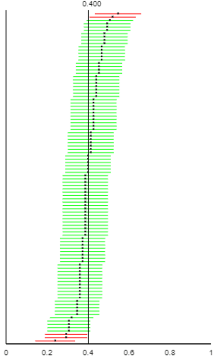
These are still approximate probabilities, but these are probably closer to the truth (meaning, closer to the theoretical long-run proportions) than our by-hand approximations, because they are based on many more repetitions (1000 instead of 96).  By clicking on the bar in the graph corresponding to 0 matches, we obtain the following graph, which shows the proportion (relative frequency) of occurrences of 0 matches as a function of the number of repetitions (trials):

I point out that this proportion bounces around quite a bit when there are a small number of trials, but the proportion seems to be settling down as the number of repetitions increases.  In fact, it’s not too much of a stretch to believe that the proportion might be approaching some limiting value in the long run.  This limiting value is what the term probability means.

Determine the approximate probability that at least one mother gets the correct baby.  Indicate two different ways to determine this.  Also interpret this (approximate) probability.  One way is to add up the number of repetitions with at least one match: (344 + 241 + 46) / 1000 = 0.631.  Another way is to subtract the estimate for 0 matches from one: 1 – 0.369 = 0.631.  Based on our simulation analysis, we estimate that at least one mother would get the correct baby in 63.1% of all repetitions, if this random process of distributing four babies to mothers at random were repeated a very large number of times.


Can we calculate the exact, theoretical probabilities here?  In other words, can we figure out the long-run limiting values for these proportions?  Yes, we can, and it’s not terribly hard.  But I don’t do this in “Stat 101” courses because I consider this to be a mathematical topic that can distract students’ attention from statistical thinking.  The essential point for statistical thinking is to think of probability as the long-run proportion of times that an event would happen if the random process were repeated a very large number of times, and I think the simulation analysis achieves this goal.

I do present the calculation of exact probabilities in introductory courses for mathematically inclined students and also in a statistical literacy course that includes a unit on randomness and probability.  The first step is to list all possible outcomes of the random process, called a sample space.  In other words, we need to list all ways to distribute four babies to their mothers at random.  This can be quite challenging and time-consuming for students who are not strong mathematically, so I present the sample space to them:

How is this list to be understood?  I demonstrate this for students by analyzing entries in the first column.  The outcome 1234 in the upper left means that all four mothers get the correct baby.  The outcome 2134 below that means that mothers 3 and 4 got the correct baby, but mothers 1 and 2 had their babies swapped.  The outcome 3124 (below the previous one) means that mother 4 got the correct baby, but mother 1 got baby 3 and mother 2 got baby 1 and mother 3 got baby 2.  The outcome 4123 in the bottom left means that all four mothers got the wrong baby: mother 1 got baby 4, and mother 2 got baby 1, and mother 3 got baby 2, and mother 4 got baby 3.

How does this list lead us to probabilities?  We take the phrase “at random” to mean that all 24 of these possible outcomes are equally likely.  Therefore, we can calculate the probability of an event by counting how many outcomes comprise the event and dividing by 24, the total number of outcomes.

Determine the number of matches for each outcome.  Then count how many outcomes produce 0 matches, 1 match, and so on.  Finally, divide by the total number of outcomes to determine the exact probabilities.  Express these probabilities as fractions and also as decimals, with three decimal places of accuracy. I ask students to work together on this and compare their answers with nearby students.  The correct answers are:

Compare these (exact) probabilities to the approximate ones from the by-hand and applet simulations.  Students notice that the simulation analyses, particularly the applet one based on a larger number of repetitions, produced reasonable approximations.

Determine and interpret the probability that at least one mother gets the correct baby.  This probability is (8+6+1)/24 = 15/24 = .625.  We could also calculate this as 1 – 9/24 = 15/24 = .625.  If this random process were repeated a very large number of times, then at least one mother would get the correct baby in about 62.25% of the repetitions.

Determine and interpret the probability that at least half of the four mothers get the correct baby.  This probability is (6+1)/24 = 7/24 ≈ .292.  This means that if this random process were repeated a very large number of times, then at least half of the mothers would get the correct baby in about 29.2% of the repetitions.

Finally, we return to the question of ordering the three events listed above, from least likely to most likely.  The correct ordering is:

  • All four of the mothers get the correct baby (probability .042).
  • None of the four mothers gets the correct baby (probability .375).
  • At least one of the four mothers gets the correct baby (probability .625).

Here are some follow-up questions that I have asked on a quiz or exam:

For parts (a) – (c), suppose that three people (Alisha, Beth, Camille) drop their cell phones in a crowded elevator.  The phones get jostled so much that each person picks up a phone at random.  The six possible outcomes can be listed (using initials) as: ABC, ACB, BAC, BCA, CAB, CBA.

  • a) The probability that all three of them pick up the correct phone can be shown to be 1/6 ≈ .167.  Does this mean that if they repeat this random process (of dropping their three phones and picking them up at random) for a total of 6 repetitions, you can be sure that all three will get the correct phone exactly once?  Answer yes or no; also explain your answer.
  • b) Determine the probability that at least one of them picks up the correct phone.  Express this probability as a fraction and a decimal.  Show your work.
  • c) Interpret what this probability means by finishing this sentence: If the random process (of three people picking up cell phones at random) were repeated a very large number of times, then …

For parts (d) – (f), suppose instead that six people in a crowded elevator drop their cell phones and pick them up at random.

  • d) Would the probability that all of the people pick up the correct phone be smaller, the same, or larger than with three people?
  • e) Which word or phrase – impossible, very unlikely, or somewhat unlikely – best describes the event that exactly five of the six people pick up the correct phone?
  • f) Which word or phrase – impossible, very unlikely, or somewhat unlikely – best describes the event that all six people pick up the correct phone?

Answers: a) No. The 1/6 probability refers to the proportion of times that all three would get the correct phone in the long run, not in a small number (such as six) of repetitions. b) There are four outcomes in which at least one person gets the correct phone (ABC, ACB, BAC, CBA), so this probability is 4/6 = 2/3 ≈ .667. c) … all three people would pick up the correct phone in about 2/3 (or about 66.7%) of the repetitions. d) Smaller e) Impossible f) Very unlikely


I like to think that this memorable context forms the basis for an effective activity that helps students to develop a basic understanding of probability as the long-run proportion of times that an event occurs.

P.S. As I’ve said before, Beth Chance deserves the lion’s share (and then some) of the credit for the applet collection that I refer to often. Carlos Lima, a former student of Beth’s for an introductory statistics course, designed and implemented the animation features in the “random babies” applet.

#16 Questions about cats

I like cats*.  I also notice that it’s simply impossible to spell STATISTICS without the letters C, A, T, and S. These two facts provide more than enough justification for me to ask many questions in class that pertain to cats in one way or another.  I believe that the upcoming questions about felines (and their human friends) can help students to learn important concepts in descriptive statistics, probability, and statistical inference**.

* This is one of the shortest sentences that I’ve ever written, even shorter than: Ask good questions.

** If you are more interested in cats than in these statistical concepts, I invite you to skip down to the P.P.S. at the end of this post to see photos of my cats.


I heard Jay Lehmann present the following question at a conference.  I liked it so much (not only because it mentions cats) that I began using it on my own final exams:

1a) Which would be larger – the average weight of 10 randomly selected people, or the average weight of 1000 randomly selected cats (ordinary domestic housecats)?

Jay mentioned that some of his students struggle with this question, because they don’t think proportionally.  They believe that the weights of 1000 cats must be larger than the weight of 10 people.  This would be true, of course, if we were talking about combined weight, but the question asks about average weight, which requires thinking on a per individual (person or cat) basis. There’s no doubt that people weigh more on average than cats.

I’m pleased to say that my students had no difficulty with this question.  But I decided to ask a second question:

1b) Which would be larger – the standard deviation of the weights of 1000 randomly selected people, or the standard deviation of the weights of 10 randomly selected cats (ordinary domestic housecats)?

The correct answer, of course, is that the standard deviation would be much larger for people than for cats, because weights of people range from just a few pounds for newborns to hundreds and hundreds of pounds for overweight adults.  Cats’ weights range only from a pound or less in kittens to a few dozen pounds for overweight cats.

My students did very poorly on this question.  Why?  I think they believe that a larger sample size produces a smaller standard deviation, period.  I never said that, of course.  What I did say, and what we investigated with simulation, is that the standard deviation of a sample mean decreases as the sample size increases.  We also explored how the standard deviation of a sample proportion decreases as the sample size increases.  We also looked at some formulas that make this more explicit, such as:

I’m afraid that many students came away from these discussions believing that “larger sample sizes produce smaller standard deviations” without paying attention to the crucial of a sample statistic part.  In an effort to curb this misunderstanding, I now try to never say or write standard deviation without adding of what for more clarity.

My students’ performance on this question is especially disheartening because I fear that a higher percentage get this wrong on the final exam than would have at the beginning of the course.  In other words, I worry that my teaching on this topic is violating the fundamental principle of “first do no harm.”

Oh dear, after a light-hearted introduction, this post has taken a discouraging turn!  Let’s move on to happier thoughts about cats (and even dogs) …


The following questions address some basic ideas of working with percentages.  You could use these to introduce, or assess students’ understanding of, probabilities of unions of events.

2. The 2018 General Social Survey (GSS) interviewed a national sample of American adults and found that 47% have a pet dog and 25% have a pet cat.

a) Does it necessarily follow that 72% (which is 47% + 25%) of those surveyed had a pet dog or a pet cat?  If not, is it even possible (in principle anyway) for this to be true?  Under what circumstance (however unrealistic) would this be true?

This conclusion does not follow, because some people have both a pet dog and a pet cat.  In other words, having a dog and having a cat are not mutually exclusive.  It’s theoretically possible that 72% of those surveyed have a pet dog or a pet cat, but this would only be true if absolutely nobody in the survey had both a dog and a cat.

b) The 2018 GSS also found that 14% of survey respondents had both a dog and a cat.  What can you conclude about the percentage who had a dog or a cat?

By adding 47% and 25%, we double-count the people who had both a dog and a cat.  We can compensate for this double-counting by subtracting off the percentage who had both.  The percentage of those surveyed who had a dog or a cat is therefore 47% + 25% – 14% = 58%.

This can be seen by putting the given percentages into the 2×2 table on the left below and then filling in the remaining percentages to produce the table on the right.  The filled-in table shows that you can calculate the percentage who had a dog or a cat by adding the three percentages in red, or else (as I did above) by adding the (marginal) percentages for each pet and then subtracting off the (joint) percentage with both pets in order to compensate for double-counting.

c) If we only knew the percentages in part (a) and not the percentage in part (b), what would be the smallest possible percentage of respondents who owned a pet dog or a pet cat?  Describe the (unrealistic) situation in which this extreme case would occur.

This question is very challenging for many students.  One way to tackle this is to start with the 2×2 table on the left below.  Then realize that to make the percentage with a dog or cat as small as possible, we need to make the percentage in the upper-left cell (with both a dog and a cat) as large as possible.  How large can that percentage be?  No larger than 25%, the percentage with a cat.  The completed table on the right shows that this extreme situation occurs only if none of the respondents had a cat and not a dog.  In other words, the most extreme case is that every person with a cat also had a dog, which gives 47% with a dog or a cat, the same as the percentage with a dog.


The following set of questions is one of my favorites (again, not only because it concerns cats).  I have long used this example to introduce students to two important ideas in statistical inference: the fundamental distinction between statistical significance and practical importance, and the consistency between confidence intervals and hypothesis tests.

3. The 2012 Statistical Abstract of the United States gives information from a national survey of 47,000 U.S. households in 2006, which found that 32.4% of the households sampled had a pet cat.  Consider this as a random sample of American households in 2006.

a) What are the observational units and variable?  What type of variable is this?

The observational units are households, not people and not cats.  The variable is whether or not the household has a cat, which is … (get ready for it) … a CATegorical variable.

b) Conduct a hypothesis test of whether the sample data provide strong evidence that the population proportion of all American households that had a pet cat in 2006 differed from one-third. Summarize your conclusion.

The z-test statistic is calculated as:

With such a large (in absolute value) z-test statistic, the p-value is very small (about 0.00002).  The sample data provide extremely strong evidence that the proportion of all American households that had a pet cat in 2006 was not one-third.

c) Produce and interpret a 99.9% confidence interval for the population proportion of all American households that own a pet cat.

This confidence interval is calculated as:

This becomes .324 ± .007, which is the interval (.317 → .331).  We can be 99.9% confident that the population proportion of American households that had a pet cat in 2006 was between .317 and .331.

Parts (a) – (c) provide fairly routine practice. The following parts introduce students to important ideas.  I encourage students to think through these questions in groups before I lead a discussion about the answers and what they’re supposed to learn from them.  I also caution students to read parts (e) and (f) very carefully to notice the small but important difference in these questions.

d) Are the test decision and confidence interval consistent with each other?  Explain.

Yes, these results are consistent.  The hypothesis test provided extremely strong evidence that the population proportion is not one-third, and the confidence interval does not include the value one-third (roughly .3333).

e) Do the sample data provide very strong evidence that the population proportion who own a pet cat is not one-third?  Explain whether the p-value or confidence interval helps you to decide.

Yes.  The p-value is extremely small (approximately .00002), so the sample data provide very strong evidence that the population proportion is not one-third.  Whatever this population proportion might equal, we have very strong evidence that it’s not one-third.

f) Do the sample data provide strong evidence that the population proportion who own a pet cat is very different from one-third?  Explain whether the p-value or confidence interval helps you to decide.

No.  The confidence interval shows us that we can be very confident that the population proportion who had a cat in 2006 is between about .317 and .331.  In other words, we can be very confident that between 31.7% and 33.1% of all American households had a pet cat in 2006.  In practical terms, this is quite close to one-third, or 33.33%.

g) What aspect of this study is responsible for the somewhat surprising pair of findings that we have very strong evidence that: (1) the population proportion is not one-third, and (2) the population proportion is quite close to one-third?

The driving factor is the very large sample size of 47,000 households. With such a large sample size, even the small difference between the sample percentage (32.4%) and the hypothesized percentage (33.33%) is enough to be statistically significant, meaning that a difference that large would be very unlikely to occur by chance alone.  The large sample size also produces a very narrow confidence interval (even with a very high confidence level), so we can be very confident that the population percentage is very close to 32.4%, which in turn is quite close to one-third in practical terms

The bottom line here is very important for students to understand about statistical inference: With a large sample size, a small difference can be statistically significant but not practically important.


Next comes a series of questions for showing how confidence intervals and hypotheses tests relate when comparing two groups and highlighting the important role of sample size in statistical inference.

4. A national survey of pet owners in the U.S. found that 53% of cat owners and 63% of dog owners said that they would perform CPR on their pets in the event of a medical emergency.

a) Are these numbers parameters or statistics?  Explain.

These numbers are statistics, because they describe the sample of dog and cat owners who were surveyed, not all dog and cat owners in the U.S.

b) State the appropriate null and alternative hypotheses for testing whether the difference between 53% and 63% is statistically significant in this context.

The null hypothesis is that the population proportions who would perform CPR on their pet are the same for dog owners and cat owners.  The alternative hypothesis is that these population proportions are different.  We could represent these hypotheses in symbols as H0: π_dog = π_cat, Ha: π_dog ≠ π_cat.

c) What additional information would you need in order to conduct a test of these hypotheses?

We need to know the sample sizes: how many dog owners and how many cat owners were surveyed?  I have to admit that I am incredibly picky when I grade student responses on this question.  If a student responds with “sample size,” that only gets partial credit. The response needs to use the plural, because learning the combined sample size is not sufficient information for conducting the test.

d) Suppose for now that the sample sizes had been 100 in each group.  Determine the z-score and p-value of the test.  Would you reject the null hypothesis at the .05 significance level?

I ask students to use technology to perform the calculations here, so they can focus on the more important concept to be addressed after part (e).  A free online tool is available here.  The test statistic turns to be z ≈ 1.43, with a two-sided p-value of 0.1520.  This p-value is greater than .05, so the observed difference in sample proportions is not statistically significant at the .05 level.

e) Determine and interpret a 95% confidence interval for the difference in the two population proportions.

Again I ask students to use technology for the calculation, which produces a 95% CI of (-0.036 → 0.236).  We can be 95% confident that the proportion of all dog owners who would perform CPR is anywhere from .036 smaller to .236 larger than the proportion of all cat owners who would perform CPR.

f) Are the test decision and confidence interval consistent with each other?  Explain how you can tell.

Yes, these results are consistent.  We did not conclude that the two groups differ, and the confidence interval (for the difference in population proportions) includes the value zero.

g) Now suppose that the sample sizes had been 500 in each group.  Determine the z-score and p-value and confidence interval.  Summarize your conclusions.

The test statistic becomes z ≈ 3.20, with a two-sided p-value of 0.0014.  The 95% CI becomes (0.039 → 0.161).  Now we do have strong evidence that dog owners and cat owners differ with regard to the population proportion who would perform CPR on their pets.  We can be 95% confident the proportion of all dog owners who would perform CPR is somewhere from .039 to .161 larger than the proportion of all cat owners who would perform CPR.

h) Describe how the p-value and confidence interval changed with the larger sample sizes.

The p-value became much smaller, enough to indicate that the difference in the observed sample proportions was unlikely to have occurred by chance alone.  The confidence interval became much narrower, enough that it contains only positive values, indicating that a higher proportion of dog owners than cat owners would perform CPR on their pet in an emergency.

The point here is to help students recognize once again the substantial role that sample size plays in statistical inference.


I promised back in post #6 (here) that I would devote a future post to nothing but questions about cats.  I am happy to check this off as a promise kept.  I hope that cat-lovers and dog-lovers alike have found something worthwhile in this post. Among their many other benefits to society, cats can help students to learn statistics!


P.S. The percentages from the GSS in question #2 came from a Washington Post article (here).  An earlier Washington Post article (here) summarized discrepancies in pet ownership estimates from different sources. The data in question #3 can be found in Table 1241 of the 2012 Statistical Abstract of the United States (here).  The survey about performing CPR on pets was summarized in a Los Angeles Times article (here).

P.P.S. I dedicate this post to the three cats who have been provided so much happiness to my wife and me.  Our first cat Eponine was a classic scaredy-cat, afraid of her own shadow.  She decided early in life that she would never do anything daring but would try to live as long as possible.  She succeeded quite well, making it to 23 years and 3 months.  On the other hand, Cosette sought adventure and lived every day to the fullest.  As a self-respecting calico cat, she became the undisputed, benevolent head of our household from the moment she joined it.  Our current cat Puti is a very good-natured boy who loves to purr, sit on laps, and complain that his 6am breakfast is served much too late in the day.

My three cats: Eponine (top left), Cosette (top right), Puti (bottom)

#15 How confident are you? part 2

How confident are you that your students can interpret a 95% confidence interval (CI) correctly?  This post continues the previous one (here) by considering numerical data and highlighting a common misconception about interpreting a CI for a population mean.

Here is the formula for a one-sample t-interval for a population mean μ, using conventional notation:

It’s worth making sure that students understand this notation.  Two quiz questions that I often ask are: 1.Remind me: what’s the difference between μ and x-bar?  2. Remind me of what the symbol s stands for, and be sure to use three words in your response.  Of course,I want students to say that μ is the symbol for a population mean and x-bar for a sample mean.  I also hope they’ll say that s stands for a sample standard deviation.  If they respond only with standard deviation, I tell them that this response is too vague and does not earn full credit.


Let’s dive in to an example that we’ll use throughout this post: I’d like to estimate the average runtime of a feature film in the thriller genre.  I selected a simple random sample of 50 thriller films from the population of 28,369* thrillers listed at IMDb (here).

* There are actually 41,774 feature films in the thriller genre listed at IMDb on October 13, 2019, but runtimes are provided for only 28,369 of them.

Consider the following (Minitab) output of the sample data:

My questions for students are:

  • (a) What are the observational units and variable?  What type of variable is this?
  • (b) Describe the relevant population and parameter.  Also indicate an appropriate symbol for this parameter.
  • (c) Identify the appropriate confidence interval procedure.
  • (d) Are the technical conditions for this procedure satisfied?  Explain.
  • (e) Calculate a 95% confidence interval for the population mean.
  • (f) Interpret this interval.
  • (g) What percentage of the films in the sample have times that fall within this interval?
  • (h) Is this percentage close to 95%?  Should it be?  Explain what went wrong, or explain that nothing went wrong.

Here are my answers:

  • (a) The observational units are the films.  The variable is the runtime of the film, measured in minutes, which is a numerical variable.
  • (b) The population is all feature films in the thriller genre listed at IMDb for which runtimes are provided.  The parameter is the mean (average) runtime among these flims, denoted by μ.
  • (c) We will use a one-sample t-interval procedure to estimate the population mean μ.
  • (d) The dotplot of the sample data reveals that the distribution of runtimes is skewed to the right.  But the skewness is not extreme, so the sample size of 50 films should be large enough for the t-interval procedure to be valid.
  • (e) The 95% CI for μ is calculated as: 101.70 ± 2.010×25.30/sqrt(50), which is 101.70 ± 7.19, which is the interval (94.51 → 108.89) minutes.
  • (f) We are 95% confident that the population mean runtime of a feature film in the thriller genre in IMDb is between 94.51 and 108.89 minutes.
  • (g) Only 7 of the 50 films (14%) run for more than 94.51 minutes and less than 108.89 minutes, as shown in red in this dotplot:
  • (h) This percentage (14%) is nowhere close to 95%.  Moreover, there’s no reason to expect this percentage to be close to 95%.  Nothing went wrong here.  Remember that the CI is estimating the population mean (average), not individual values.  We do not expect 95% of the individual films’ runtimes to be within this CI.  Rather, we are 95% confident that the population mean of the runtimes is within this CI.

Question (h) indicates a very common and troublesome student misconception.  Many students mistakenly believe that a 95% CI for a population mean is supposed to contain 95% of the data values.  These students are confusing confidence about a parameter with prediction about an individual.  How can we help them to see the mistake here?  I hope that questions (g) and (h) help with this, as students should see for themselves that only 7 of the 50 films (14%) in this sample fall within the CI.  You might also point out that as the sample size increases, the CI for μ will continue to get narrower, so the interval will include fewer and fewer data values.  We can also be sure to ask students to identify parameters in words as often as possible, because I think this misconception goes back to not paying enough attention to what a parameter is in the first place.

Something else we could consider doing* to help students to distinguish between confidence and prediction is to teach them about prediction intervals, which estimate individual values rather than the population mean.  In many situations the relevant question is one of prediction.  For example, you might be much more interested in predicting how long the next thriller film that you watch will take, as opposed to wanting to estimate how long a thriller film lasts on average.

* I confess that I do not typically do this, except in courses for mathematically inclined students such as those majoring in statistics, mathematics, or economics.

Here is the formula for a prediction interval:

Comparing this to the confidence interval formula above, we see that the prediction interval formula has an extra s (sample standard deviation) term. This accounts for variability from individual to individual, which makes the prediction interval much wider than the confidence interval.  For the sample data on runtimes of thriller films, the 95% prediction interval is: 101.70 ± 2.010×25.30×sqrt(1+1/50), which is 101.70 ± 51.36, which is the interval (50.34 → 153.06) minutes.  Notice how wide this interval is: Its half-width is 51.36 minutes (nearly an hour), compared to a half-width of just 7.19 minutes for the confidence interval above.  This prediction interval captures 45 of the 50 runtimes in this sample (90%).

An important caveat is that unlike the t-confidence interval procedure for a population mean, this prediction interval procedure relies heavily on the assumption of a normally distributed population, regardless of sample size.  The runtime distribution is skewed to the right, so this t-prediction interval procedure is probably not valid.  A simpler alternative is to produce a prediction interval by using the (approximate) 2.5th and 97.5th percentiles of the sample data.  For this sample, we could use the second-smallest and second-largest runtime values, which gives a prediction interval of (60 → 163) minutes.  This interval contains 48/50 (96%) of the runtimes in the sample.


Now let’s re-consider question (f), which asked for an interpretation of the confidence interval.  Below are four possible student answers.  As you read these, please think about whether or not you would award full credit for that interpretation:

  • 1. We are 95% confident that μ is between 94.5 and 108.9.
  • 2. We are 95% confident that the population mean is between 94.5 and 108.9 minutes.
  • 3. We are 95% confident that the population mean runtime of a thriller film in the IMDb list is between 94.5 and 108.9 minutes.
  • 4. We are 95% confident that the population mean runtime of a thriller film in the IMDb list is between 94.5 and 108.9 minutes.  This confidence stems from knowing that 95% of all confidence intervals generated by this procedure would succeed in capturing the actual value of the population mean.

I hope we agree that none of these interpretations is flat-out wrong, and they get progressively better as we progress from #1 through #4.  Where would you draw the line about deserving full credit?  I would regard #3 as good enough.  I think #1 and #2 fall short by not providing context.  I view #4 as going beyond what’s needed because the question asked only for an interpretation of the interval, not for the meaning of the 95% confidence level.  I suggest asking a separate question specifically about interpreting confidence level*, in order to assess students’ understanding of that concept.

* I have asked: Explain what the phrase “95% confidence” means in this interpretation. This is a challenging question for most students.


Continuing this deep dive into into interpreting a confidence interval for a population mean, please consider the following incorrect answers.  Think about which you consider to be more or less serious than others, and also reflect on which interpretations deserve full credit, partial credit, or no credit.

  • A. We are 95% confident that a thriller film in the IMDb list runs for between 94.5 and 108.9 minutes.
  • B. There’s a 95% chance that a thriller film in the IMDb list runs for between 94.5 and 108.9 minutes.
  • C. About 95% of all thriller films in the IMDb list run for between 94.5 and 108.9 minutes.
  • D. We are 95% confident that the mean runlength of a thriller film in this sample from the IMDb list was between 94.5 and 108.9 minutes.
  • E. We are 95% confident that the mean runlength of a thriller film in a new random sample from the IMDb list would be between 94.5 and 108.9 minutes.
  • F. There’s a 95% chance (or a 0.95 probability) that the population mean runlength of a thriller film in the IMDb list is between 94.5 and 108.9 minutes.

I contend that A, B, and C are all egregiously wrong.  They all make the same mistake of thinking that the interval predicts the runtime of individual films rather than estimating a mean.  I suppose you could say that A is better than B and C because it uses the word “confident.” In fact, simply inserting “on average” at the end of the sentence would be sufficient to fix A.  But the idea of “on average” is a crucial one to have omitted!

I believe that D and E are slightly less wrong than A, B, and C, because they do include the idea of mean.  But they refer to a sample mean instead of the population mean.  This is also a serious error and so would receive no credit in my class.  I might say that D is worse than E, because we know for sure that the mean runtime in this sample is the midpoint of the confidence interval.

What about F?  It’s not quite correct, because it uses the language of chance and probability rather than confidence.  The population mean μ is a fixed value, so it’s not technically correct* to refer to the probability or chance that μ falls in a particular interval.  What’s random is the confidence interval itself, because the interval obtained from this procedure would vary from sample to sample if we were to take repeated random samples from the population**.  But I consider this distinction between confidence and probability to be fairly minor, especially compared to the much more substantive distinction between confidence and prediction.  I would nudge a student who produced F toward more appropriate language but would award full credit for this interpretation.

* Unless we take a Bayesian approach, which I will discuss in a future post.

** As we saw in the previous post (here) by using the Simulating Confidence Intervals applet (here).


I ask a version of the “do you expect 95% of the data to fall within the CI” question almost every time I ask about interpreting a confidence interval.  I remember one student from many years ago who seemed to be either tickled or annoyed by my repeating this question so often.  In response to such a question on the final exam, he wrote something like: “Boy, some students must get this wrong a lot because you keep asking about it.  Okay, once again, my answer is …”  You might be expecting me to conclude this post on an ironic note by saying that the student then proceeded to give a wrong answer.  But no, he nailed it.  He knew that we do not expect anywhere near 95% of the data values to fall within a 95% confidence interval for the population mean.  I hope that this student would be tickled, and not annoyed, to see that I have now devoted most of a blog post to this misconception.

P.S. The sample data on runtimes can be found in the file below.

#14 How confident are you? part 1

How confident are you that your students understand what “95% confidence” means?  Or that they realize why we don’t always use 99.99% confidence?  That they can explain the sense in which larger samples produce “better” confidence intervals than smaller samples?  For that matter, how confident are you that your students know what a confidence interval is trying to estimate in the first place?  This blog post, and the next one as well, will focus on helping students to understand basic concepts of confidence intervals. (As always, my questions to students appear in italics below.)


I introduce confidence intervals (CIs) to my students with a CI for a population proportion, using the conventional method given by:

Let’s apply this to a surveyed that we encountered in post #8 (here) about whether the global rate of extreme poverty has doubled, halved, or remained about the same over the past twenty years.  The correct answer is that the rate has halved, but 59% of a random sample of 1005 adult Americans gave the (very) wrong answer that they thought the rate had doubled (here). 

Use this sample result to calculate a 95% confidence interval.  This interval turns out to be:

This calculation becomes .59 ± .03, which is the interval (.56, .62)*.  Interpret what this confidence interval means.  Most students are comfortable with concluding that we are 95% confident that something is between .56 and .62.  The tricky part is articulating what that something is.  Some students mistakenly say that we’re 95% confident that this interval includes the sample proportion who believe that the global poverty rate has doubled.  This is wrong, in part because we know that the sample proportion is the exact midpoint of this interval.  Other students mistakenly say that if researchers were to select a new sample of 1005 adult Americans, then we’re 95% confident that between 56% and 62% of those people would answer “doubled” to this question.  This is incorrect because it is again trying to interpret the confidence interval in terms of a sample proportion.  The correct interpretation needs to make clear what the population and parameter are: We can be 95% confident that between 56% and 62% of all adult Americans would answer “doubled” to the question about how the global rate of extreme poverty has changed over the past twenty years.

* How are students supposed to know that this (.56, .62) notation represents an interval?  I wonder if we should use notation such as (.56 → .62) instead?

Now comes a much harder question: What do we mean by the phrase “95% confident” in this interpretation?  Understanding this concept requires thinking about how well the confidence interval procedure would perform if it were applied for a very large number of samples.  I think the best way to explore this is with … (recall from the previous post here that I hope for students to complete this sentence with a joyful chorus of a single word) … simulation!


To conduct this simulation, we use one of my favorite applets*.  The Simulating Confidence Intervals applet (here) does what its name suggests:

  • simulates selecting random samples from a probability distribution,
  • generates a confidence interval (CI) for the parameter from each simulated sample,
  • keeps track of whether or not the CI successfully captures the value of the population parameter, and
  • calculates a running count of how many (and what percentage of) intervals succeed.

* Even though this applet is one of my favorites, it only helps students to learn if you … (wait for it) … ask good questions!

The first step in using the applet is to specify that we are dealing with a proportion, sampling from a binomial model, and using the conventional z-interval, also known as the Wald method:

The next step is to specify the value of the population proportion.  The applet needs this information in order to produce simulated samples, but it’s crucial to emphasize to students that you would not know the value of the population proportion in a real study.  Indeed, the whole point of selecting a random sample and calculating a sample proportion is to learn something about the unknown value of the population proportion.  But in order to study properties of the CI procedure, we need to specify the value of the population proportion.  Let’s use the value 0.40; in other words we’ll assume that 40% of the population has the characteristic of interest.  Let’s make this somewhat more concrete and less boring: Suppose that we are sampling college students and that 40% of college students have a tattoo.  We also need to enter the sample size; let’s start with samples of n = 75 students.  Let’s generate just 1 interval at first, and let’s use 95% confidence:

Here’s what we might observe* when we click the “Sample” button in the applet:

* Your results will vary, of course, because that’s the nature of randomness and simulation.

The vertical line above the value 0.4 indicates that the parameter value is fixed.  The black dot is the value of the simulated sample proportion, which is also the midpoint of the interval (0.413* in this case).  The confidence interval is shown in green, and the endpoint values (0.302 → 0.525) appear when you click on the interval.  You might ask students to use the sample proportion and sample size to confirm the calculation of the interval’s endpoints.  You might also ask students to suggest why the interval was colored green, or you might ask more directly: Does this interval succeed in capturing the value of the population proportion (which, you will recall, we stipulated to be 0.4)?  Yes, the interval from 0.302 to 0.525 does include the value 0.4, which is why the interval was colored green.

* This simulated sample of 75 students must have included 31 successes (with a tattoo) and 44 failures, producing a sample proportion of 31/75 ≈ 0.413).

At this point I click on “Sample” several times and ask students: Does the value of the population proportion change as the applet generates new samples?  The answer is no, the population proportion is still fixed at 0.4, where we told the applet to put it.  What does vary from sample to sample?  This a key question.  The answer is that the intervals vary from sample to sample.  Why do the intervals vary from sample to sample?  Because the sample proportion, which is the midpoint of the interval, varies from sample to sample.  That’s what the concept of sampling variability is all about.

I continue to click on “Sample” until the applet produces an interval that appears in red, such as:

Why is this interval red?  Because it fails to capture the value of the population proportion.  Why does this interval fail when most succeed?  Because random chance produced an unusually small value of the sample proportion (0.253), which led to a confidence interval (0.155 → 0.352) that falls entirely below the value of the population proportion 0.40.

Now comes the fun part and a pretty picture.  Instead of generating one random sample at a time, let’s use the applet to generate 100 samples/intervals all at once.  We obtain something like:

This picture captures what the phrase “95% confidence” means.  But it still takes some time and thought for students to understand what this shows.  Let’s review:

  • The applet has generated 100 random samples from a population with a proportion value of 0.4.
  • For each of the 100 samples, the applet has used the usual method to calculate a 95% confidence interval.
  • These 100 intervals are displayed with horizontal line segments.
  • The 100 sample proportions are represented by the black dots at the midpoints of the intervals.
  • The population proportion remains fixed at 0.4, as shown by the vertical line. 
  • The confidence intervals that are colored green succeed in capturing the value 0.4.
  • The red confidence intervals fail to include the value 0.4.

Now, here’s the key question: What percentage of the 100 confidence intervals succeed in capturing the value of the population proportion?  It’s a lot easier to count the red ones that fail: 5 out of 100.  Lo and behold, 95% of the confidence intervals succeed in capturing the value of the population proportion.  That is what “95% confidence” means.

The applet also has an option to sort the intervals, which produces:

This picture illustrates why some confidence intervals fail: The red intervals were the unlucky ones with an unusually small or large value of the sample proportion, which leads to a confidence interval that falls entirely below or above the population proportion value of 0.4.

A picture like this appears in many statistics textbooks, but the applet makes this process interactive and dynamic.  Next I keep pressing the “Sample” button in order to generate many thousands of samples and intervals.  The running total across thousands of samples should reveal that close to 95% of confidence intervals succeed in capturing the value of the population parameter.

An important question to ask next brings this idea back to statistical practice: Survey researchers typically select only one random sample from a population, and then they produce a confidence interval based on that sample.How do we know whether the resulting confidence interval is successful in capturing the unknown value of the population parameter?  The answer is that we do not know.  This answer is deeply unsatisfying to many students, who are uncomfortable with this lack of certainty.  But that’s the unavoidable nature of the discipline of statistics.  Some are comforted by this follow-up question: If we can’t know for sure whether the confidence interval contains the value of the population parameter, on what grounds can we be confident about this?  Our 95% confidence stems from knowing that the procedure produces confidence intervals that succeed 95% of the time in the long run.  That’s what the large abundance of green intervals over red ones tells us.  In practice we don’t know where the vertical line for the population value is, so we don’t know whether our one confidence interval deserves to be colored green or red, but we do know that 95% of all intervals would be green, so we can be 95% confident that our interval deserves to be green.


Whew, that’s a lot to take in!  But I must confess that I’m not sure that this long-run interpretation of confidence level is quite as important as we instructors often make it out to be.  I think it’s far more important that students be able to describe what they are 95% confident of: that the interval captures the unknown value of the population parameter.  Both of those words are important – population parameter – and students should be able to describe both clearly in the context of the study.

I can think of at least three other aspects of confidence intervals that I think are more important (than the long-run interpretation of confidence level) for students to understand well.


1. Effect of confidence level – why don’t we always use 99.99% confidence?

Let’s go back to the applet, again with a sample size of 75.  Let’s consider changing the confidence level from 95% to 99% and then to 80%.  I strongly encourage asking students to think about this and make a prediction in advance: How do you expect the intervals to change with a larger confidence level?  Be sure to cite two things that will change about the intervals.  Once students have made their predictions, we use the applet to explore what happens:

99% confidence on the left, 80% confidence on the right

The results for 99% confidence are on the left, with 80% confidence on the right.  A larger confidence level produces wider intervals and a larger percentage of intervals that succeed in capturing the parameter value.  Why do we not always use 99.99% confidence?  Because those intervals would typically be so wide as to provide very little useful information*.

* Granted, there might be some contexts for which this level of confidence is necessary.  A very large sample size could prevent the confidence interval from becoming too wide, as the next point shows.


2. Effect of sample size – in what sense do larger samples produce better confidence intervals than smaller samples? Let’s return to the applet with a confidence level of 95%.  Now I ask: Predict what will change about the intervals if we change the sample size from 75 to 300.  Comment on both the intervals’ widths and the percentage of intervals that are successful.  Most students correctly predict that the larger sample size will produce intervals that are more narrow.  But many students mistakenly predict that the larger ample size will result in a higher percentage of successful intervals.  Results such as the following (n = 75 on the left, n = 300 on the right) convince them that they are correct about narrower intervals, but the percentage of successful ones remains close to 95%, because that is controlled by the confidence level:

n = 75 on the left, n = 300 on the right

This graph (and remember that students using the applet would see many such graphs dynamically, rather than simply seeing this static image) confirms students’ intuition that a larger sample size produces narrower intervals.  That’s the sense in which larger sample sizes produce better confidence intervals, because narrower intervals indicate a more precise (i.e., better) estimate of the population parameter for a given confidence level.

Many students are surprised, though, to see that the larger sample size does not affect the green/red breakdown.  We should still expect about 95% of confidence intervals to succeed in capturing the population proportion, for any sample size, because we kept the confidence level at 95%.


3. Limitations of confidence intervals – when should we refuse to calculate a confidence interval?

Suppose that an alien lands on earth and wants to estimate the proportion of human beings who are female*.  Fortunately, the alien took a good statistics course on its home planet, so it knows to take a sample of human beings and produce a confidence interval for this proportion.  Unfortunately, the alien happens upon the 2019 U.S. Senate as its sample of human beings.  The U.S. Senate has 25 women senators (its most ever!) among its 100 members in 2019.

* I realize that this context is ridiculous, but it’s one of my favorites.  In my defense, the example does make use of real data.

a) Calculate the alien’s 95% confidence interval.  This interval is:

This calculation becomes .25 ± .085, which is the interval (.165 → .335).

b) Interpret the interval.  The alien would be 95% confident that the proportion of all humans on earth who are female is between .165 and .335.

c) Is this consistent with your experience living on this planet?  No, the actual proportion of humans who are female is much larger than this interval, close to 0.5.

d) What went wrong?  The alien did not select a random sample of humans.  In fact, the alien’s sampling method was very biased toward under-representing females.

e) As we saw with the applet, about 5% of all 95% confidence intervals fail to capture the actual value of the population parameter.  Is that the explanation for what went wrong here?  No!  Many students are tempted to answer yes, but this explanation about 5% of all intervals failing is only relevant when you have selected random samples over and over again.  The lack of random sampling is the problem here.

f) Would it be reasonable for the alien to conclude, with 95% confidence, that between 16.5% and 33.5% of U.S. senators in the year 2019 are female?  No.  We know (for sure, with 100% confidence) that exactly 25% of U.S. senators in 2019 are female.  If that’s the entire population of interest, there’s no reason to calculate a confidence interval.  This question is a very challenging one, for which most students need a nudge in the right direction.

The lessons of this example are:

  • Confidence intervals are not appropriate when the data were collected with a biased sampling method.  A confidence interval calculated from such a sample can provide very dubious and misleading information.
  • Confidence intervals are not appropriate when you have access to the entire population of interest.  In this unusual and happy circumstance, you should simply describe the population.

I feel a bit conflicted as I conclude this post.  I have tried to convince you that the Simulating Confidence Intervals applet provides a great tool for leading students to explore and understand what the challenging concept of “95% confidence” really means.  But I also have also aimed to persuade you that many instructors over-emphasize this concept at the expense of more important things for students to learn about confidence intervals.

I will continue this discussion of confidence intervals in the next post, moving on to numerical variables and estimating a population mean.