Archive for

#82 Power, part 3

This post continues and completes my discussion of introducing students to the concept of power.  Let me remind you of the scenario that I presented in the first post of this series (here):

Suppose that Tamika is a basketball player whose probability of successfully making a free throw has been 0.6.  During one off-season, she works hard to improve her probability of success.  Of course, her coach wants to see evidence of her improvement, so he asks her to shoot some free throws.  If Tamika really has improved, how likely is she to convince the coach that she has improved?

The first post in this series described using an applet (here) to conduct simulation analyses to lead students to the concepts of rejection region and power, and then to consider factors that affect power.  In this post I will make three points about teaching these concepts in courses for mathematically inclined students, such as those majoring in statistics or mathematics or engineering or economics.

---

1. Start with simulation analyses, even for mathematically inclined students.

I suspect that some statistics teachers regard simulation as a valuable tool for students who are uncomfortable with math but not necessarily with mathematically inclined students.  I agree I think simulation can be very enlightening and powerful tools even with students who enjoy and excel at mathematical aspects of statistics.  I recommend introducing students to the concept of power through simulation analyses, regardless of how well prepared or comfortable the students are with mathematics.

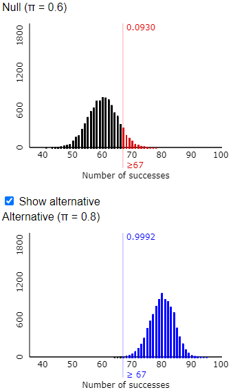
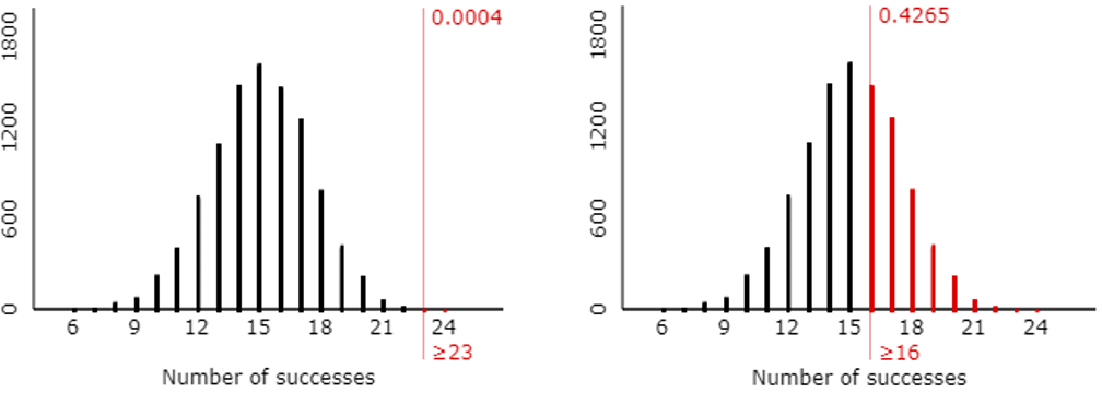
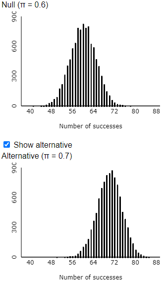
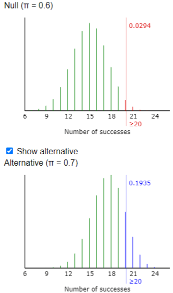
You could ask students to write their own code to conduct these simulations, but I typically stick with the applet because it’s so convenient and produces nice visuals such as:

---

2. Proceed to ask mathematically inclined students to perform probability calculations to confirm what the simulations reveal.

Tamika’s example provides a great opportunity for students to practice working with the binomial distribution:

• a) Let the random variable X represent the number of shots that Tamika would successfully make out of 25 shots, assuming that she has not improved.  What probability distribution would X have?
• b) Determine the smallest value of k for which Pr(X ≥ k) ≤ 0.05.
• c) Does this agree with your finding from the simulation analysis?
• d) Explain what this number has to do with Tamika’s efforts to convince the coach that she has improved.

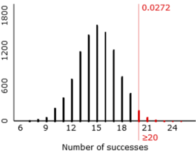
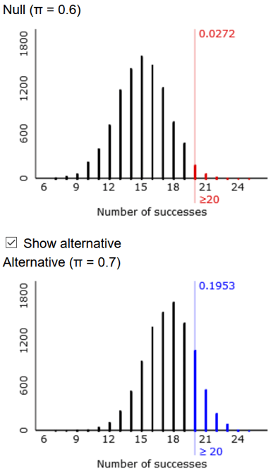
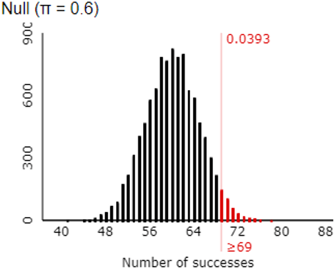
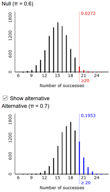
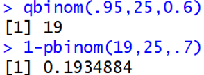
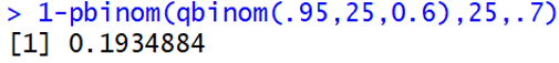
The random variable X would have a binomial distribution with n = 25 and p = 0.6.  To answer part (b), students could work with a cumulative distribution function by realizing that Pr(X ≥ k) = 1 – Pr(X ≤ k – 1) in this case.  Then they can use software or a graphing calculator to determine that the smallest value of k that satisfies this criterion is k = 20, for which Pr(X ≥ 20) ≈ 0.0294.  This means that Tamika must successfully make 20 or more of the 25 shots to convince her coach that she has improved, when the coach gives her 25 shots and using 0.05 as his standard to be convinced.

Instead of using the cumulative distribution function, students could use the inverse cumulative distribution function built into many software programs.  For example, this command in R is:

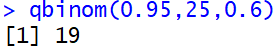
Some students get tripped up by the need for the first input to be 0.95 rather than 0.05.  Students also need to be careful to realize that the output value of 19 = k – 1, so the value of k = 20.  As some students struggle with this, I remind them of two things: First, they should return to their simulation results to make sure that their binomial calculations agree.  Second, when they’re not sure whether 19 or 20 is the answer they’re looking for, they can check that by calculating Pr(X ≥ 19) and Pr(X ≥ 20) to see which one meets the criterion.

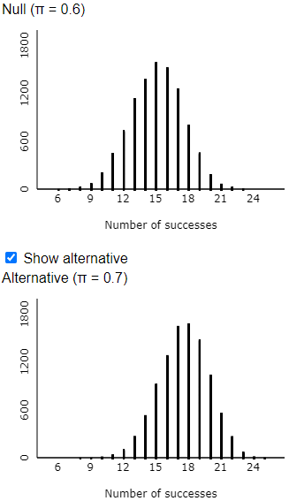
• e) Let the random variable Y represent the number of shots that Tamika would successfully make if she has improved her success probability to 0.7.  What probability distribution would Y have?
• f) Determine Pr(Y ≥ k) for the value of k that you determined in part (b).
• g) Does this agree with your finding from the simulation analysis?
• h) Explain what this number has to do with Tamika’s efforts to convince the coach that she has improved.

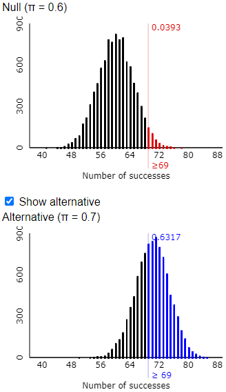
The random variable Y would have a binomial distribution with n = 25 and p = 0.7.  Once they realize this, students can use software to calculate Pr(Y ≥ 20) ≈ 0.1935.  For example, the R command to calculate this is:

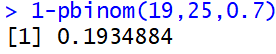
This probability is very close to the approximation from the simulation analysis.  Tamika has slightly less than a 20% chance of convincing her coach that she has improved, if she is given a sample of 25 shots, the coach uses a significance level of 0.05, and her improved probability of success is 0.7 rather than 0.6.

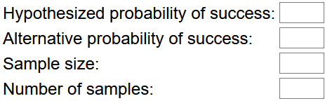
Students can then use software to produce exact power calculations, using the binomial probability distribution, for different values of the sample size, significance level, and improved success probability.

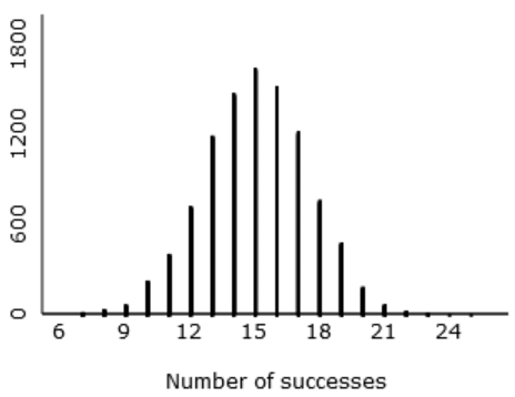
A drawback of using software such as R or Excel to calculate these probabilities is that they do not automatically provide visual representation of the probability distribution.  The applet that I used for the simulation analyses does have an option to calculate and display exact binomial probabilities:

---

3. Ask mathematically inclined students to write code to produce graphs of power as a function of sample size, or significance level, and of alternative value for the parameter.

Recall that the pair of R commands for calculating the rejection region and power for Tamika’s first situation is:

Then I like to ask mathematically included students: Re-write this power calculation to use just one line of code.  For students who need a hint: Where did the 19 value in the second line come from?  This leads to:

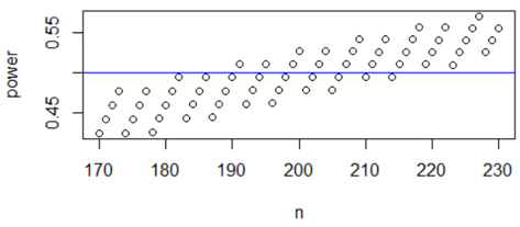
A follow-up is: How can you alter this command to calculate power as a function of sample size, for values from n = 1 through n = 300?  The key is to replace the value 25 with a vector (call it n) containing integer values from 1 through 300.  The resulting graph (with α = 0.05 and p_alt = 0.7) is:

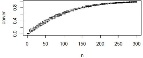
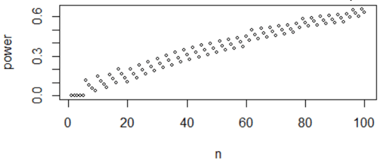
Does this graph behave as you expected?  Mostly yes, but there’s an oddity.  This graph shows that power generally increases as sample size increases, as we expected.  But I say generally because there are lots of short-run exceptions, because of the discrete-ness of the binomial distribution.  The pattern is more noticeable if we restrict our attention to sample sizes values from n = 1 through 100:

Students can then proceed to produce and describe graphs of power as a function of significance level and of the improved probability value (for n = 25 in both graphs, p_alt = 0.7 on the left, and α= 0.05 on the right), as shown here:

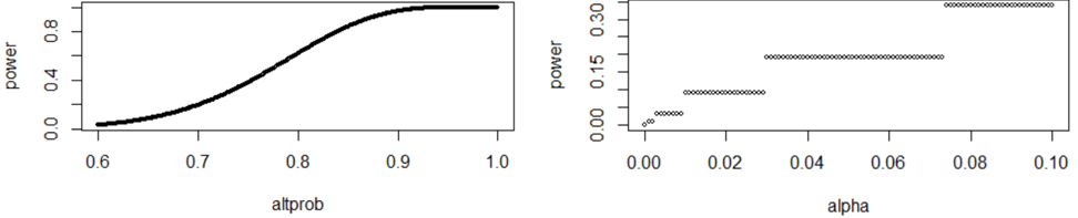
Do these graphs behave as you expected?  Power increases as the significance level increases, as expected, but this is a step function due to the discreteness.  Power does increase as the improved probability value increases, as expected.

---

The concept of power is a challenging one for many students to grasp.  I recommend starting with a simple scenario involving a single proportion, such as Tamika trying to convince her coach of her improvement as a free throw shooter.  I think simulation analyses and visualizations can help students to understand the key ideas*.  With mathematically inclined students, I suggest following up the simulations with probability calculations and simple coding as described in this post. My hope is that these activities deepen their understanding of power and also their facility with probability distributions.

* As long as the simulation analyses are accompanied by asking good questions!

#81 Power, part 2

In last week’s post (here), I presented an extended series of questions that used a simulation analysis to introduce students to the concept of statistical power.  The simulation analysis used an applet (here) to produce graphs like this:

In the context of last week’s example, this pair of graphs shows that there’s about a 63% that Tamika will perform well enough to convince her coach that she has improved, based on a sample size of 100 shots, a significance level of 0.05, and an improvement in her probability of success from 0.6 to 0.7.

Needless to say, I believe that the questions I presented can be helpful for developing students’ understanding of the concept of power.  I hasten* to add that this activity is far from fool-proof.  In this post, I will discuss a few common difficulties and misunderstandings.

* Well, it took me a week, so perhaps I have not really hastened to add this, but I like the sound of the word.

---

A big part of my point in last week’s post was that we can help students to focus on the concept of power by postponing the use of statistical terminology.  I waited until we had completed the simulation activity before defining the terms power and also type I error and type II error.  Of course, this required me to move beyond simply talking about whether Tamika had improved or not, and whether her coach was convinced or not.  At this point I mentioned terms such as null hypothesis and alternative hypothesis, rejecting the null hypothesis and failing to reject the null hypothesis.  Then I asked my students to state the null and alternative hypotheses that Tamika’s coach was testing, both in words and in terms of a parameter. 

Most students seemed to realize quickly that the null hypothesis was that Tamika had not improved, and the alternative was that she had improved.  But they struggled with expressing these hypotheses in terms of a parameter.  To point them in the right direction, I asked whether the parameter is a proportion or a mean, but this did not seem to help.  I took a conceptual step back and asked whether the variable is categorical or numerical.  This time several students answered quickly but incorrectly in the zoom chat that the variable was numerical. 

This is a very understandable mistake, because graphs such as the ones above display the distribution of a numerical variable.  But I pointed out that the variable for Tamika is whether or not she successfully makes a shot, which is categorical.  The parameter is therefore the long-run proportion of shots that she would make, which my students know to represent with the symbol π.  The hypotheses are therefore H₀: π = 0.6 (no improvement) versus H_a: π > 0.6 (improvement).

This difficulty reveals a common problem when using simulation to introduce students to concepts of statistical inference.  To understand what the simulation analysis and resulting graphs reveal, it’s crucial to realize that such graphs are not displaying the results not of a single sample, which is what we would observe in practice.  Rather, the graphs are showing results for a large number of made-up samples, under certain assumptions, in order to investigate how the procedure would perform in the long run.  This is a big conceptual leap.  I strongly recommend using physical devices such as coins and cards for students’ first encounters with simulation (see posts #12 and #27, here and here), in order to help them with recognizing this step and taking it gradually.  When you rely on technology to conduct simulations later, students must follow this step in their minds to make sense of the results.

---

As I presented the activity for my students via zoom, I also encouraged them to use the applet to carry out simulation analyses themselves.  I should not have been surprised by the most common question I received from my students, but I was surprised at the time.  Several students expressed concern about getting slightly different values than I did.  For example, they might have gotten 0.6271 or 0.6343 rather than the 0.6317 that I obtained in the graphs above.  I responded that this was a good question but nothing to worry about.  Those differences, I said, were due to the random nature of simulation and therefore to be expected.  I added that using a large number of repetitions for the simulation analysis, such as 10,000, should ensure that we all obtain approximately the same value.

Some students followed up by asking how such responses will be graded on assignments and exams.  I had been thinking that some students resist a simulation-based approach because they are uncomfortable with approximate answers rather than a single correct answer.  But this question made me realize that some students may be skeptical of simulation analyses not for intellectual or psychological reasons but rather out of concern about their grades.

I tried to assure my students that with simulation analyses, reasonable values in the right ballpark would earn full credit, for both open-ended and auto-graded responses.  I should have also thought to respond that many questions will instead ask about the simulation process and the interpretation of results.

---

My pledge that students would receive full credit for reasonable approximations was called into question less than half an hour after class ended.  Here are the questions that I asked in the (auto-graded) follow-up quiz:

Suppose that I have regularly played Solitaire on my computer with a 20% chance of winning any one game.  But I have been trying hard lately to improve my probability of winning, and now I will play a series of (independent) games to gather data for testing whether I have truly improved.

1. What is the alternative hypothesis to be tested?  [Options: That I have improved; That I have not improved; That I have doubled my probability of winning a game]

2. Suppose that I have not improved, but the data provide enough evidence to conclude that I have improved.  What type of error would this represent?  [Options: Type I error; Type II error; Type III error; Standard error]

Now suppose that I really have improved, and my success probability is now 25% rather than 20%.  Also suppose that I plan to play 40 independent games and that my test will use a significance level of 0.05.  Use the Power Simulation applet to conduct a simulation analysis of this situation.

3. What is the rejection region of the test?  [Options: Winning 13 or more times in the 40 games; Winning 20 or more times in the 40 games; Winning 8 or more times in the 40 games; Winning 10 or more times in the 40 games]

4. Which of the following comes closest to the probability that these 40 games will provide convincing evidence of my improvement?  [Options 0.18; 0.25; 0.40; 0.75; 0.99]

5. Continue to assume that my success probability is now 25% rather than 20% and that the test uses a significance level of 0.05.  About how many games would I have to play in order to have a 50% chance that the games will provide convincing evidence of my improvement?  Enter your answer as an integer.  (Hint: Use the applet, and feel free to use trial-and-error.) 

For questions #3 and #4, I spaced the options far enough apart to leave no doubt about the correct answers, as long as the student conducted the simulation correctly and used a reasonably large number of repetitions.  Question #5 is the most interesting and problematic one.  Asking students to determine a sample size that would achieve a particular value of power went a bit beyond what we had done in the class activity.  Students were supposed to realize that increasing sample size generally increases power, and I gave them the hint to feel free to use trial-and-error.  I thought I had allowed for a reasonably large interval of answers to receive full (auto-graded) credit, but a student came to my virtual office hours to ask why her answer had not received credit.  She showed me that her sample size did indeed produce a power value close to 0.5, so I expanded the interval of values to receive full credit*. I also let her know that I greatly appreciate students who begin assignments early and draw concerns to my attention quickly.

* The discrete-ness of the binomial distribution is more of an issue here than variability of simulation results.  I will discuss this further in part 3 of this series, but for now I’ll show a graph of power (calculated from the binomial distribution) as a function of sample size for the values that I decided to accept as reasonable.  This graph shows that power does generally increase with sample size, but the discrete-ness here makes the function more interesting and non-monotonic:

---

I believe that the simulation activity that I presented last week is effective for introducing students to the concept of power.  But I also acknowledge that this is a challenging topic, so in this post I have tried to point out some difficulties that students encounter.

#80 Power, part 1

I wish I had a better title for this post.  This one-word title reminds me of my two-part post about confounding variables, which I simply titled Confounding (see posts #43 and #44, here and here).  I tried to be clever with that title by arguing that the concept of confounding is one of the most confounding topics that students encounter in introductory statistics.  I suppose I could argue that the concept of power is one of the most powerful topics that students encounter, but my point is really that power is another topic that students find to be especially confounding.  I will abandon my search for cleverness and stick with this boring (but not misleading!) title.

I think we can help students to understand the concept of power by eliminating unnecessary terminology and calculations for our first pass at the topic.  We don’t need to mention null and alternative hypotheses, or rejection regions, or Type I and Type II errors, or p-values, or binomial or normal distributions, or expected value or standard deviation or z-score.  Don’t get me wrong: We’ll use most of those ideas, but we don’t need to let the terminology get in the way.

Instead we can present students with a scenario and an overarching question that you and I recognize as a question of power.  Then we can lead students to answer that big question by asking a series of smaller questions.  Questions that I pose to students appear in italics below.

---

Here’s the scenario that I use with my students: Suppose that Tamika is a basketball player whose probability of successfully making a free throw has been 0.6.  During one off-season, she works hard to improve her probability of success.  Of course, her coach wants to see evidence of her improvement, so he asks her to shoot some free throws. 

Here’s the overarching question: If Tamika really has improved, how likely is she to convince the coach that she has improved?  The other big question is: What factors affect how likely she is to convince the coach that she has improved?

I try not to over-do sports examples with my students, but I think the context here is very helpful and easy to follow, even for students who are not sports fans.

You won’t be surprised to see that we’ll use simulation as our tool to address these questions.

---

Let’s say that the coach gives Tamika 25 shots with which to demonstrate her improvement.

a) Suppose that she successfully makes 23 of the 25 shots.  Would you be reasonably convinced that she has improved?  Why or why not?

b) What if she makes 16 of the 25 shots – would you be reasonably convinced that she has improved?  Why or why not?

Most students realize that 60% of 25 is 15*, so both 16 and 23 are more successes that we would expect (for the long-run average) if she had not improved.  Their intuition suggests that 23 successes would provide very strong evidence of improvement, because it seems unlikely that a 60% shooter would achieve that many successes.  On the other hand, 16 successes does not provide strong evidence of improvement, because it seems that a 60% shooter could easily get a bit lucky and obtain 16 successes.

* You’re welcome to call this the expected value if you’d like.

c) What does your intuition suggest about how many shots Tamika would have to make successfully in order to be convincing? 

When I asked my students to type their answer to this question into the zoom chat during class a few days ago, nearly every student typed 20.  I said that this seemed reasonable and that we would proceed to use simulation to investigate this question a bit more carefully.  We used an applet (here) to conduct the simulation analysis.  The applet inputs required are:

d) Which input values can you specify already?

The hypothesized probability of success is 0.6, and the sample size is 25.  Later we’ll assume that Tamika has improved to have a 70% chance of success, so we’ll enter 0.7 for the alternative probability of success.  I like to start with simulating just one sample at a time, so we’ll enter 1 for number of samples at first; later we’ll enter a large number such as 10,000 for the number of samples.

e) Click on “draw samples” five times, using 1 for the number of samples each time.  Did each of the simulated samples produce the same number of successful shots?

Part e) would be easy to skip, but I think it’s important.  This question forces students to acknowledge randomness, or sampling variability.  I don’t think any students struggle to answer this correctly, but I think it’s worth drawing their attention to this point.

f) Now enter 9995 for the number of samples, and click on “draw samples” to produce a total of 10,000 simulated sample results.  Describe the resulting distribution for the number of successes.  Comment on shape, center, and variability.

Here are some typical results:

My students are quick to say that the shape of this distribution is symmetric, unimodal, normal-ish.  The center is near 15, which is what we expected because 60% of 25 is 15.  There’s a good bit of variability here: The simulated results show that Tamika sometimes made as few as 7 or 8 shots out of 25, and she also made as many as 23 or 24 shots out of 25.

g) Has this simulation analysis assumed that Tamika has improved, or that Tamika has not improved?

This is also a key question that is easy for students to miss: This simulation analysis has assumed that Tamika has not improved*.  We use the distribution of the number of successes, assuming that she has not improved, to decide how many successes she needs to provide convincing evidence of improvement.  I try to reinforce this point with the next question:

* You’re welcome to call this the null hypothesis.

h) Based on these simulation results, do you feel justified in your earlier answers about whether 23 successes, or 16 successes, would provide convincing evidence of improvement?  Explain.

Students who thought that 23 successes in 25 attempts provides very strong evidence of improvement should feel justified, because this simulation reveals that such an extreme result would happen only about 4 times in 10,000* (see graph on the left).  Similarly, students were correct to believe that 16 successes does not provide much evidence of improvement, because it’s not at all unlikely (better than a 40% chance*) for a 60% shooter to do that well (or better) by random chance (see graph on the right).

* You’re welcome to refer to these percentages as approximate p-values.  See post #12 (here) for an introduction to simulation-based inference.

---

Now we come to one of the harder questions:

i) Suppose that the coach decides on the following criterion for his decision rule: He’ll decide that Tamika has improved if her number of successes is large enough that such an extreme result would happen less than 5% of the time with a 60% shooter.  According to this rule, how many shots does Tamika need to make successfully to convince her coach?

I encourage students to answer this at first with trial-and-error.  Enter 17, and then 18, and so on into the “rejection region” box until you find the smallest number for which less than 5% of the simulated samples produce such a large number (or more) of successes.  The answer turns out to be that Tamika needs to make 20 or more of the 25 shots* to be convincing, as shown here:

* You’re welcome to call this the rejection region of the test, especially as the applet uses that term.

I was quick to point out to my students how good their intuition was.  As I mentioned earlier, nearly all of my students who responded in the zoom chat predicted that Tamika would need to make 20 shots to be convincing.

Now, finally, we address the big picture question:

j) Make a guess for how likely Tamika is to make 20 or more shots successfully out of 25 attempts, if she has improved to a 0.7 probability of successfully making a single shot.

I don’t really care how well students guess here.  My point is to remind them of the big question, the reason we’re going through all of this.  Next we use the applet to conduct another simulation to answer this question:

k) Check the “show alternative” box in the applet, which displays the distribution of number of successes, assuming that Tamika has improved to a 0.7 probability of success.  Do you see much overlap in the two distributions?  Is this good news or bad news for Tamika?  Explain.

There is considerable overlap in the two distributions, as shown here:

l) According to the applet’s simulation results, in what percentage of the 10,000 simulated samples does Tamika, with a 70% chance of making a single shot, do well enough to convince the coach of her improvement by successfully making 20 or more shots?  Would you say that Tamika has a good chance of demonstrating her improvement in this case?

Unfortunately for Tamika, she does not have a good chance of demonstrating her improvement.  In my simulation result shown here, she only does so about 19.5% of the time:

Here’s where we introduce the term of the day: We have approximated the power of this test.  Power in this case represents the probability that Tamika convinces her coach that she has improved, when she truly has improved.

---

Now we’ll begin to consider factors that affect power, first by asking:

m) What would you encourage Tamika to request, in order to have a better chance of convincing the coach that she has improved?

Several of my students responded very quickly in the zoom chat to say: more shots*.

* You’re welcome to call this a larger sample size.

n) Now suppose that the coach offers 100 shots for Tamika to show her improvement.  Re-run the simulation analysis.  Is there more, less, or the same amount of overlap in the two distributions?  Is this good news or bad news for Tamika?  Explain.

The simulation results reveal that the larger sample size leads to much less overlap between these two distributions:

This is very good news for Tamika, because this shows that it’s easier to distinguish a 70% shooter from a 60% shooter when she takes 100 shots than with only 25 shots.

o) How many shots must she now make successfully in order to convince the coach?  How does this compare to the percentage of 25 shots that she needs to make in order to be convincing?

The following graph shows that making 69 or more shots is sufficient to convince the coach that she has improved from a 60% shooter:

Recall that with 25 shots, Tamika had to make 20 of them to be convincing, so the percentage that she needs to make has decreased from 80% to 69% with the increase in sample size.

p) What is the (approximate) probability that Tamika will be able to convince the coach of her improvement, based on a sample of 100 shots?  How has this changed from the earlier case in which she could only take 25 shots?

This output shows that she has about a 63% chance of convincing the coach now:

This probability is more than three times larger than the previous case with only 25 shots.

q) What else could Tamika ask the coach to change about his decision process, in order to have a better chance to convince him of her improvement?

This one is much harder for students to suggest than sample size, but someone eventually proposes to change the 5% cut-off value, the significance level.  Making that larger would mean that the coach is requiring less strong evidence to be convincing, so that will increase Tamika’s chances of convincing the coach.

r) Change the coach’s significance level from 0.05 to 0.10.  How does this change the number of shots that Tamika must make to convince the coach of her improvement?  How does this change the probability that she convinces the coach of her improvement?

As shown in the following output, Tamika now only needs to make 67 shots, rather than 69, in order to convince the coach.  The probability that she achieves this as a 70% shooter is approximately 0.777, which is considerably larger than the previous probability of approximately 0.632.

s) Identify one more factor that affects how likely Tamika is to convince the coach that she has improved.

I sometimes give a hint by suggesting that students think about the applet’s input values. Then someone will suggest that Tamika could try to improve more.

t) Now suppose that Tamika improves so much that she has a 0.8 probability of successfully making a single shot.  How does this change the number of shots that Tamika must make to convince the coach of her improvement?  How does this change the probability that she convinces the coach of her improvement?

I tell students that they do not need to use the applet to answer the first of these questions.  This change does not affect how many shots she must make to convince the coach.  That value depends only on her previous probability of success, not her new and improved probability of success.  But her new success probability will produce even greater separation between the two distributions and will increase her probability of convincing the coach.  The following output reveals that the new probability is approximately 0.999:

---

This activity can introduce students to the concept of power without burdening them with too much terminology or too many calculations.  I grant that it’s very convenient to use terms such as significance level and rejection region and power, but I prefer to introduce those after students have first explored the basic ideas.

In the second post in this series, I will discuss some common questions from students, describe some assessment questions that I used for this topic, including some that I now regret, and present extensions of this activity for introducing the concept of power to more mathematically inclined students.

#79 No blog post today

I’m sorry to report that I do not have a blog post for today.

Hold on – doesn’t that sentence itself, especially when combined with this one, constitute a blog post?!  After all, you can see for yourself that I am posting this on my blog. 

But while this may constitute a logical puzzle, or conundrum, or paradox, it’s not really related to teaching introductory statistics, and it does not ask good questions, so I don’t know that you should consider this a legitimate blog post.  I am only sending this out because some of you have been very nice to say that you look forward to hearing from me on Monday mornings, so I thought I should announce and explain that I have no blog post this week.

The explanation is simply that I’ve fallen behind, and today (Mon Jan 4) is the first day of classes for the Winter quarter at Cal Poly, and I’ve needed to spend my time on preparing for class rather than writing a blog post.

I will be teaching the second course in our two-course sequence for Business majors.  The first course included basic ideas of data collection and analysis, a good bit of probability, and statistical inference for one variable.  After a brief review, this second course entails inference for comparing groups, chi-square tests, analysis of variance, simple linear regression, and multiple regression.  For good measure, the course concludes with brief introductions to time series and quality control.

This will be my second experience teaching an entirely online course.  I’m feeling less nervous than I was at the start of the Fall quarter, but I also feel that this time I should set my sights higher than simply surviving the experience.

I have mentioned before that I give lots of quizzes to my students.  I have already posted three quizzes before my class even begins.  One is about a welcome video that I prepared, another about a video that introduces myself to students (which I wrote about in post #63, titled My first video, here), and a third about the course syllabus.  I tell students that these quizzes essentially offer free points, because students are welcome to re-watch the videos and re-read the syllabus after they have seen the quiz questions. 

Just for fun, here are some of the questions on these quizzes*:

1. Which of the following is NOT a reasonable description of statistics?  [Options: Confusing people with nonsense; gaining insights from data; Making decisions under uncertainty]
2. How many quizzes will we have?  [Options: A few; Lots; None]
3. How should you interact with your classmates and instructor?  [Options: With arrogance and condescension; With courtesy and respect; With rudeness and sarcasm]
4. Are you responsible for practicing academic honesty?  [Options: No; Only on odd-numbered dates; Only on Sundays; Yes]
5. What is my teaching philosophy?  [Options: Ask good questions; Insist on perfection; Learn by viewing; Rely on luck]

* I usually report the answers to my quiz questions, but this time I think I’ll trust you to figure them out for yourself.

I apologize in advance in case I need to return to “no blog post today” a few times in the coming weeks, but I will definitely return.  Some topics that I have in mind include introducing students to the concept of power and questioning whether two-sided tests are always preferable to one-sided ones.  I will also write about one of my favorite topics to teach, one that does not often come up in statistics courses but is especially relevant when teaching Business students: adjusting for inflation.

Best wishes for asking good questions in 2021!

P.S. Hey, wait a minute – did I just write a blog post today after all? [Options: Absolutely; Not even close; Well, kind of]