#14 How confident are you? part 1

How confident are you that your students understand what “95% confidence” means?  Or that they realize why we don’t always use 99.99% confidence?  That they can explain the sense in which larger samples produce “better” confidence intervals than smaller samples?  For that matter, how confident are you that your students know what a confidence interval is trying to estimate in the first place?  This blog post, and the next one as well, will focus on helping students to understand basic concepts of confidence intervals. (As always, my questions to students appear in italics below.)

---

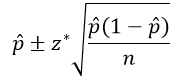
I introduce confidence intervals (CIs) to my students with a CI for a population proportion, using the conventional method given by:

Let’s apply this to a surveyed that we encountered in post #8 (here) about whether the global rate of extreme poverty has doubled, halved, or remained about the same over the past twenty years.  The correct answer is that the rate has halved, but 59% of a random sample of 1005 adult Americans gave the (very) wrong answer that they thought the rate had doubled (here). 

Use this sample result to calculate a 95% confidence interval.  This interval turns out to be:

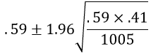
This calculation becomes .59 ± .03, which is the interval (.56, .62)*.  Interpret what this confidence interval means.  Most students are comfortable with concluding that we are 95% confident that something is between .56 and .62.  The tricky part is articulating what that something is.  Some students mistakenly say that we’re 95% confident that this interval includes the sample proportion who believe that the global poverty rate has doubled.  This is wrong, in part because we know that the sample proportion is the exact midpoint of this interval.  Other students mistakenly say that if researchers were to select a new sample of 1005 adult Americans, then we’re 95% confident that between 56% and 62% of those people would answer “doubled” to this question.  This is incorrect because it is again trying to interpret the confidence interval in terms of a sample proportion.  The correct interpretation needs to make clear what the population and parameter are: We can be 95% confident that between 56% and 62% of all adult Americans would answer “doubled” to the question about how the global rate of extreme poverty has changed over the past twenty years.

* How are students supposed to know that this (.56, .62) notation represents an interval?  I wonder if we should use notation such as (.56 → .62) instead?

Now comes a much harder question: What do we mean by the phrase “95% confident” in this interpretation?  Understanding this concept requires thinking about how well the confidence interval procedure would perform if it were applied for a very large number of samples.  I think the best way to explore this is with … (recall from the previous post here that I hope for students to complete this sentence with a joyful chorus of a single word) … simulation!

---

To conduct this simulation, we use one of my favorite applets*.  The Simulating Confidence Intervals applet (here) does what its name suggests:

• simulates selecting random samples from a probability distribution,
• generates a confidence interval (CI) for the parameter from each simulated sample,
• keeps track of whether or not the CI successfully captures the value of the population parameter, and
• calculates a running count of how many (and what percentage of) intervals succeed.

* Even though this applet is one of my favorites, it only helps students to learn if you … (wait for it) … ask good questions!

The first step in using the applet is to specify that we are dealing with a proportion, sampling from a binomial model, and using the conventional z-interval, also known as the Wald method:

The next step is to specify the value of the population proportion.  The applet needs this information in order to produce simulated samples, but it’s crucial to emphasize to students that you would not know the value of the population proportion in a real study.  Indeed, the whole point of selecting a random sample and calculating a sample proportion is to learn something about the unknown value of the population proportion.  But in order to study properties of the CI procedure, we need to specify the value of the population proportion.  Let’s use the value 0.40; in other words we’ll assume that 40% of the population has the characteristic of interest.  Let’s make this somewhat more concrete and less boring: Suppose that we are sampling college students and that 40% of college students have a tattoo.  We also need to enter the sample size; let’s start with samples of n = 75 students.  Let’s generate just 1 interval at first, and let’s use 95% confidence:

Here’s what we might observe* when we click the “Sample” button in the applet:

* Your results will vary, of course, because that’s the nature of randomness and simulation.

The vertical line above the value 0.4 indicates that the parameter value is fixed.  The black dot is the value of the simulated sample proportion, which is also the midpoint of the interval (0.413* in this case).  The confidence interval is shown in green, and the endpoint values (0.302 → 0.525) appear when you click on the interval.  You might ask students to use the sample proportion and sample size to confirm the calculation of the interval’s endpoints.  You might also ask students to suggest why the interval was colored green, or you might ask more directly: Does this interval succeed in capturing the value of the population proportion (which, you will recall, we stipulated to be 0.4)?  Yes, the interval from 0.302 to 0.525 does include the value 0.4, which is why the interval was colored green.

* This simulated sample of 75 students must have included 31 successes (with a tattoo) and 44 failures, producing a sample proportion of 31/75 ≈ 0.413).

At this point I click on “Sample” several times and ask students: Does the value of the population proportion change as the applet generates new samples?  The answer is no, the population proportion is still fixed at 0.4, where we told the applet to put it.  What does vary from sample to sample?  This a key question.  The answer is that the intervals vary from sample to sample.  Why do the intervals vary from sample to sample?  Because the sample proportion, which is the midpoint of the interval, varies from sample to sample.  That’s what the concept of sampling variability is all about.

I continue to click on “Sample” until the applet produces an interval that appears in red, such as:

Why is this interval red?  Because it fails to capture the value of the population proportion.  Why does this interval fail when most succeed?  Because random chance produced an unusually small value of the sample proportion (0.253), which led to a confidence interval (0.155 → 0.352) that falls entirely below the value of the population proportion 0.40.

Now comes the fun part and a pretty picture.  Instead of generating one random sample at a time, let’s use the applet to generate 100 samples/intervals all at once.  We obtain something like:

This picture captures what the phrase “95% confidence” means.  But it still takes some time and thought for students to understand what this shows.  Let’s review:

• The applet has generated 100 random samples from a population with a proportion value of 0.4.
• For each of the 100 samples, the applet has used the usual method to calculate a 95% confidence interval.
• These 100 intervals are displayed with horizontal line segments.
• The 100 sample proportions are represented by the black dots at the midpoints of the intervals.
• The population proportion remains fixed at 0.4, as shown by the vertical line. 
• The confidence intervals that are colored green succeed in capturing the value 0.4.
• The red confidence intervals fail to include the value 0.4.

Now, here’s the key question: What percentage of the 100 confidence intervals succeed in capturing the value of the population proportion?  It’s a lot easier to count the red ones that fail: 5 out of 100.  Lo and behold, 95% of the confidence intervals succeed in capturing the value of the population proportion.  That is what “95% confidence” means.

The applet also has an option to sort the intervals, which produces:

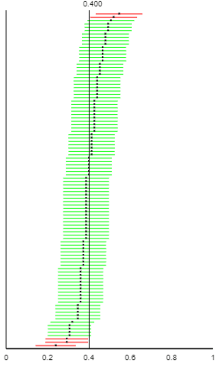
This picture illustrates why some confidence intervals fail: The red intervals were the unlucky ones with an unusually small or large value of the sample proportion, which leads to a confidence interval that falls entirely below or above the population proportion value of 0.4.

A picture like this appears in many statistics textbooks, but the applet makes this process interactive and dynamic.  Next I keep pressing the “Sample” button in order to generate many thousands of samples and intervals.  The running total across thousands of samples should reveal that close to 95% of confidence intervals succeed in capturing the value of the population parameter.

An important question to ask next brings this idea back to statistical practice: Survey researchers typically select only one random sample from a population, and then they produce a confidence interval based on that sample.How do we know whether the resulting confidence interval is successful in capturing the unknown value of the population parameter?  The answer is that we do not know.  This answer is deeply unsatisfying to many students, who are uncomfortable with this lack of certainty.  But that’s the unavoidable nature of the discipline of statistics.  Some are comforted by this follow-up question: If we can’t know for sure whether the confidence interval contains the value of the population parameter, on what grounds can we be confident about this?  Our 95% confidence stems from knowing that the procedure produces confidence intervals that succeed 95% of the time in the long run.  That’s what the large abundance of green intervals over red ones tells us.  In practice we don’t know where the vertical line for the population value is, so we don’t know whether our one confidence interval deserves to be colored green or red, but we do know that 95% of all intervals would be green, so we can be 95% confident that our interval deserves to be green.

---

Whew, that’s a lot to take in!  But I must confess that I’m not sure that this long-run interpretation of confidence level is quite as important as we instructors often make it out to be.  I think it’s far more important that students be able to describe what they are 95% confident of: that the interval captures the unknown value of the population parameter.  Both of those words are important – population parameter – and students should be able to describe both clearly in the context of the study.

I can think of at least three other aspects of confidence intervals that I think are more important (than the long-run interpretation of confidence level) for students to understand well.

---

1. Effect of confidence level – why don’t we always use 99.99% confidence?

Let’s go back to the applet, again with a sample size of 75.  Let’s consider changing the confidence level from 95% to 99% and then to 80%.  I strongly encourage asking students to think about this and make a prediction in advance: How do you expect the intervals to change with a larger confidence level?  Be sure to cite two things that will change about the intervals.  Once students have made their predictions, we use the applet to explore what happens:

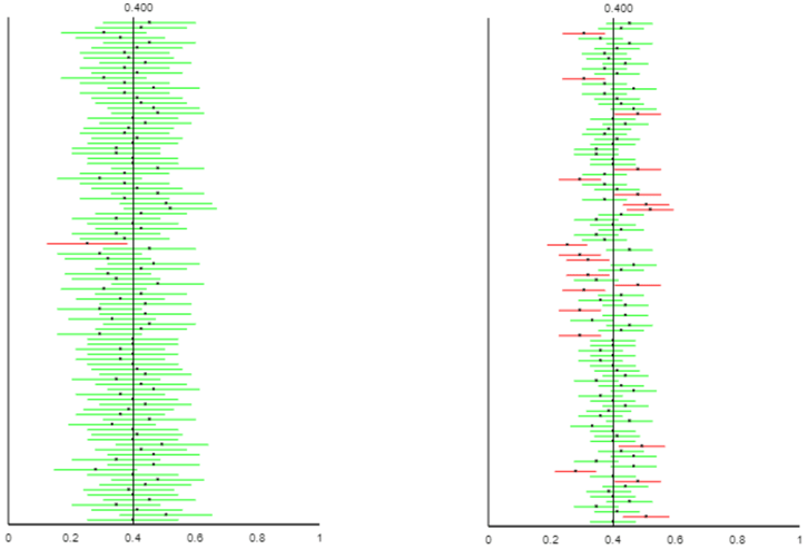
The results for 99% confidence are on the left, with 80% confidence on the right.  A larger confidence level produces wider intervals and a larger percentage of intervals that succeed in capturing the parameter value.  Why do we not always use 99.99% confidence?  Because those intervals would typically be so wide as to provide very little useful information*.

* Granted, there might be some contexts for which this level of confidence is necessary.  A very large sample size could prevent the confidence interval from becoming too wide, as the next point shows.

---

2. Effect of sample size – in what sense do larger samples produce better confidence intervals than smaller samples? Let’s return to the applet with a confidence level of 95%.  Now I ask: Predict what will change about the intervals if we change the sample size from 75 to 300.  Comment on both the intervals’ widths and the percentage of intervals that are successful.  Most students correctly predict that the larger sample size will produce intervals that are more narrow.  But many students mistakenly predict that the larger ample size will result in a higher percentage of successful intervals.  Results such as the following (n = 75 on the left, n = 300 on the right) convince them that they are correct about narrower intervals, but the percentage of successful ones remains close to 95%, because that is controlled by the confidence level:

This graph (and remember that students using the applet would see many such graphs dynamically, rather than simply seeing this static image) confirms students’ intuition that a larger sample size produces narrower intervals.  That’s the sense in which larger sample sizes produce better confidence intervals, because narrower intervals indicate a more precise (i.e., better) estimate of the population parameter for a given confidence level.

Many students are surprised, though, to see that the larger sample size does not affect the green/red breakdown.  We should still expect about 95% of confidence intervals to succeed in capturing the population proportion, for any sample size, because we kept the confidence level at 95%.

---

3. Limitations of confidence intervals – when should we refuse to calculate a confidence interval?

Suppose that an alien lands on earth and wants to estimate the proportion of human beings who are female*.  Fortunately, the alien took a good statistics course on its home planet, so it knows to take a sample of human beings and produce a confidence interval for this proportion.  Unfortunately, the alien happens upon the 2019 U.S. Senate as its sample of human beings.  The U.S. Senate has 25 women senators (its most ever!) among its 100 members in 2019.

* I realize that this context is ridiculous, but it’s one of my favorites.  In my defense, the example does make use of real data.

a) Calculate the alien’s 95% confidence interval.  This interval is:

This calculation becomes .25 ± .085, which is the interval (.165 → .335).

b) Interpret the interval.  The alien would be 95% confident that the proportion of all humans on earth who are female is between .165 and .335.

c) Is this consistent with your experience living on this planet?  No, the actual proportion of humans who are female is much larger than this interval, close to 0.5.

d) What went wrong?  The alien did not select a random sample of humans.  In fact, the alien’s sampling method was very biased toward under-representing females.

e) As we saw with the applet, about 5% of all 95% confidence intervals fail to capture the actual value of the population parameter.  Is that the explanation for what went wrong here?  No!  Many students are tempted to answer yes, but this explanation about 5% of all intervals failing is only relevant when you have selected random samples over and over again.  The lack of random sampling is the problem here.

f) Would it be reasonable for the alien to conclude, with 95% confidence, that between 16.5% and 33.5% of U.S. senators in the year 2019 are female?  No.  We know (for sure, with 100% confidence) that exactly 25% of U.S. senators in 2019 are female.  If that’s the entire population of interest, there’s no reason to calculate a confidence interval.  This question is a very challenging one, for which most students need a nudge in the right direction.

The lessons of this example are:

• Confidence intervals are not appropriate when the data were collected with a biased sampling method.  A confidence interval calculated from such a sample can provide very dubious and misleading information.
• Confidence intervals are not appropriate when you have access to the entire population of interest.  In this unusual and happy circumstance, you should simply describe the population.

---

I feel a bit conflicted as I conclude this post.  I have tried to convince you that the Simulating Confidence Intervals applet provides a great tool for leading students to explore and understand what the challenging concept of “95% confidence” really means.  But I also have also aimed to persuade you that many instructors over-emphasize this concept at the expense of more important things for students to learn about confidence intervals.

I will continue this discussion of confidence intervals in the next post, moving on to numerical variables and estimating a population mean.