#46 How confident are you? Part 3

How confident are you that your students can explain:

• Why do we use a t-distribution (rather than the standard normal z-distribution) to produce a confidence interval for a population mean? 
• Why do we check a normality condition, when we have a small sample size, before calculating a t-interval for a population mean? 
• Why do we need a large enough sample size to calculate a normal-based confidence interval for a population proportion?

I suspect that my students think we invent these additional complications – t instead of z, check normality, check sample size – just to torment them.  It’s hard enough to understand what 95% confidence means (as I discussed in post #14 here), and that a confidence interval for a mean is not a prediction interval for a single observation (see post #15 here).

These questions boil down to asking: What goes wrong if we use a confidence interval formula when the conditions are not satisfied?  If nothing bad happens when the conditions are not met, then why do we bother checking conditions?  Well, something bad does happen.  That’s what we’ll explore in this post.  Once again we’ll use simulation as our tool.  In particular, we’ll return to an applet called Simulating Confidence Intervals (here).  As always, questions for students appear in italics.

---

1. Why do we use a t-distribution, rather than a z-distribution, to calculate a confidence interval for a population mean? 

It would be a lot easier, and would seem to make considerable sense, just to plug in a z-value, like this*:

* I am using standard notation: x-bar for sample mean, s for sample standard deviation, n for sample size, and z* for a critical value from a standard normal distribution.  I often give a follow-up group quiz in which I simply ask students to describe what each of these four symbols means, along with μ.

Instead we tell students that we need to use a different multiplier, which comes from a completely different probability distribution, like so:

Many students believe that we do this just to make their statistics course more difficult.  Other students accept that this adjustment is necessary for some reason, but they figure that they are incapable of understanding why.

We can inspire better reactions than these.  We can lead students to explore what goes wrong if we use the z-interval and how the t-interval solves the problem.  As we saw in post #14 (here), the key is to use simulation to explore how confidence intervals behave when we randomly generate lots and lots of them (using the applet here).

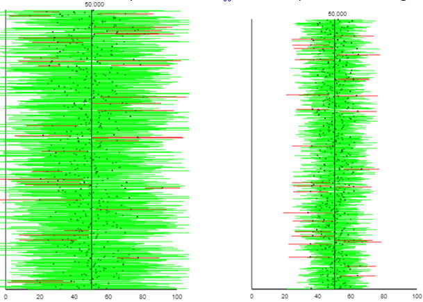
To conduct this simulation, we need to assume what the population distribution looks like.  For now let’s assume that the population has a normal distribution with mean 50 and standard deviation 10.  We’ll use a very small sample size of 5, a confidence level of 95%, and we’ll simulate selecting 500 random samples from the population.  Using the first formula above (“z with s”), the applet produces output like this:

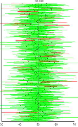
The applet reports that 440 of these 500 intervals (88.0%, the ones colored green) succeed in capturing the population mean.  The success percentage converges to about 87.8% after generating tens and hundreds of thousands of these intervals.  I ask students:

• What problem with the “z with s” confidence interval procedure does this simulation analysis reveal?  A confidence level of 95% is supposed to mean that 95% of the confidence intervals generated with the procedure succeed in capturing the population parameter, but the simulation analysis reveals that this “z with s” procedure is only succeeding about 88% of the time.
• In order to solve this problem, do we need the intervals to get a bit narrower or wider?  We need the intervals to get a bit wider, so some of the intervals that (barely) fail to include the parameter value of 50 will include it.
• Which of the four terms in the formula – x-bar, z*, s, or n – can we alter to produce a wider interval?  In other words, which one does not depend on the data?  The sample mean, sample standard deviation, and sample size all depend on the data.  We need to use a different multiplier than z* to improve this confidence interval procedure.
• Do we want to use a larger or smaller multiplier than z*?  We need a slightly larger multiplier, in order to make the intervals a bit wider.

At this point I tell students that a statistician named Gosset, who worked for Guinness brewery, determined the appropriate multiplier, based on what we call the t-distribution.  I also say that:

• The t-distribution is symmetric about zero and bell-shaped, just like the standard normal distribution.
• The t-distribution has heavier tails (i.e., more area in the tails) than the standard normal distribution.
• The t-distribution is actually an entire family of distributions, characterized by a number called its degrees of freedom (df).
• As the df gets larger and larger, the t-distribution gets closer and closer to the standard normal distribution.
• For a confidence interval for a population mean, the degrees of freedom is one less than the sample size: n – 1.

The following graph displays the standard normal distribution (in black) and a t-distribution with 4 degrees of freedom (in blue).  Notice that the blue curve has heavier tails than the black one, so capturing the middle 95% of the distribution requires a larger critical value.

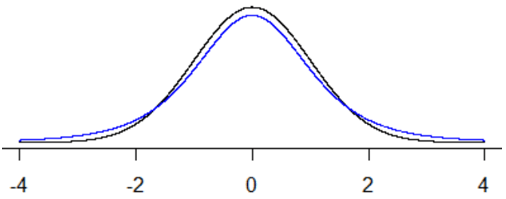
With a sample size of 5 and 95% confidence, the critical value turns out to be t* = 2.776, based on 4 degrees of freedom.  How does this compare to the value of z* for 95% confidence?  Students know that z* = 1.96, so the new t* multiplier is considerably larger, which will produce wider intervals, which means that a larger percentage of intervals will succeed in capturing the value of the population mean.

That’s great that the new t* multiplier produces wider intervals, but: How can we tell whether this t* adjustment is the right amount to produce 95% confidence?  That’s easy: Simulate!  Here is the result of taking the same 500 samples as above, but using the t-interval rather than the z-interval:

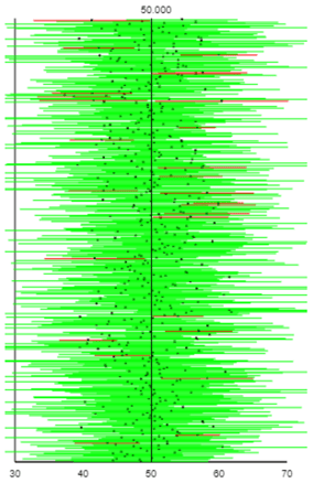
How do these intervals compare to the previous ones?  We can see that these intervals are wider.  Do more of them succeed in capturing the parameter value?  Yes, more are green, and so fewer are red, than before.  In fact, 94.6% of these 500 intervals succeed in capturing the value of 50 that we set for the population mean.  Generating many thousands more samples and intervals reveals that the long-run success rate is very close to 95.0%.

What happens with larger sample sizes?  Ask students to explore this with the applet.  They’ll find that the percentage of successful intervals using the “z with s” method increases as the sample size does, but continues to remain less than 95%.  The coverage success percentages increase to approximately 93.5% with a sample size of n = 20, 94.3% with n = 40, and 94.7% with n = 100.  With the t-method, these percentages hover near 95.0% for all sample sizes.

Does t* work equally well with other confidence levels?  You can ask students to investigate this with simulation also.  They’ll find that the answer is yes.

By the way, why do the widths of these intervals vary from sample to sample?  I like this question as a check on whether students understand what the applet is doing and how these confidence interval procedures work.  The intervals have different widths because the value of the sample standard deviation (s in the formulas above) varies from sample to sample.

Remember that this analysis has been based on sampling from a normally distributed population.  What if the population follows a different distribution?  That’s what we’ll explore next …

---

2. What goes wrong, with a small sample size, if the normality condition is not satisfied?

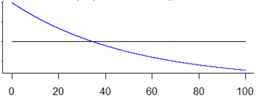
Students again suspect that we want them to check this normality condition just to torment them.  It’s very reasonable for them to ask what bad thing would happen if they (gasp!) use a procedure even when the conditions are not satisfied.  Our strategy for investigating this will come as no surprise: simulation!  We’ll simulate selecting samples, and calculating confidence intervals for a population mean, from two different population distributions: uniform and exponential.  A uniform distribution is symmetric, like a normal distribution, but is flat rather than bell-shaped.  In contrast, an exponential distribution is sharply skewed to the right.  Here are graphs of these two probability distributions (uniform in black, exponential in blue), both with a mean of 50:

The output below displays the resulting t-intervals from simulating 500 samples from a uniform distribution with sample sizes of 5 on the left, 20 on the right:

For these 500 intervals, the percentages that succeed are 92.8% on the left, 94.4% on the right.  Remind me: What does “succeed” mean here?  I like to ask this now and then, to make sure students understand that success means capturing the actual value (50, in this case) of the population mean.  I went on to use R to simulate one million samples from a uniform distribution with these sample sizes.  I found success rates of 93.4% with n = 5 and 94.8% with n = 20.  What do these percentages suggest?  The t-interval procedure works well for data from a uniform population even with samples as small as n = 20 and not badly even with sample sizes as small as n = 5, thanks largely to the symmetry of the uniform distribution.

Sampling from the highly-skewed exponential distribution reveals a different story.  The following output comes from sample sizes (from left to right) of 5, 20, 40, and 100:

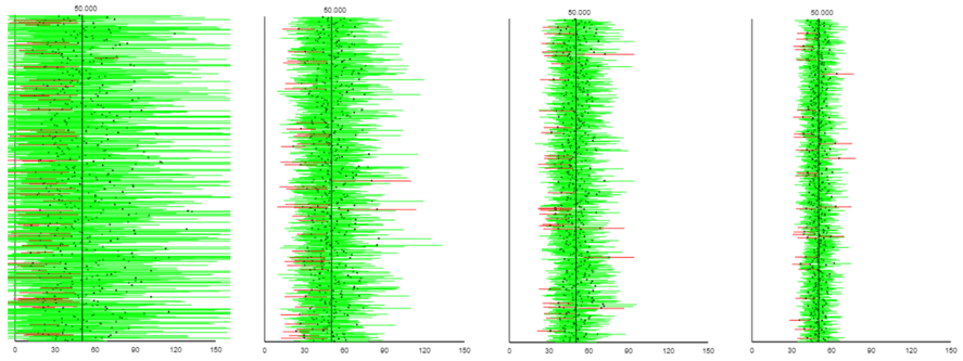
The rates of successful coverage in these graphs (again from left to right) are 87.8%, 92.2%, 93.4%, and 94.2%.  The long-run coverage rates are approximately 88.3%, 91.9%, 93.2%, and 94.2%.  With sample data from a very skewed population, the t-interval gets better and better with larger sample sizes, but still fails to achieve its nominal (meaning “in name only”) confidence level even with a sample size as large as 100.

The bottom line, once again, is that when the conditions for a confidence interval procedure are not satisfied, that procedure will successfully capture the parameter values less often than its nominal confidence level.  How much less often depends on the sample size (smaller is worse) and population distribution (more skewed is worse). 

Also note that there’s nothing magical about the number 30 that is often cited for a large enough sample size.  A sample size of 5 from a uniform distribution works as well as a sample size of 40 from an exponential distribution, and a sample size of 20 from a uniform distribution is comparable to a sample size of 100 from an exponential distribution.

Next we’ll shift gears to explore a confidence interval for a population proportion rather than a population mean …

---

3. What goes wrong when the sample size conditions are not satisfied for a confidence interval for a population proportion?

The conventional method for estimating a population proportion π is*:

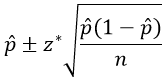
* I adhere to the convention of using Greek letters for parameter values, so I use π (pi) for a population proportion.

We advise students not to use this procedure with a small sample size, or when the sample proportion is close to zero or one.  A typical check is that the sample must include at least 10 “successes” and 10  “failures.”  Can students explain why this check is necessary?  In other words, what goes wrong if you use this procedure when the condition is not satisfied?  Yet again we can use simulation to come up with an answer.

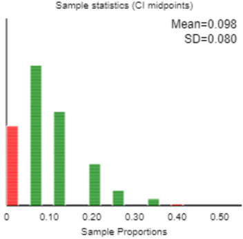
Let’s return to the applet (here).  Now we’ll select Proportions, Binomial, and the Wald method (which is one of the names for the conventional method above).  Let’s use a sample size of n = 15 and a population proportion of π = 0.1.  Here is some output for 500 simulated samples and the resulting confidence intervals:

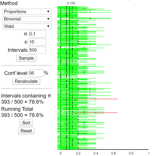
Something weird is happening here.  I only see two red intervals among the 500, yet the applet reports that only 78.6% of these intervals succeeded in capturing the value of the population proportion (0.1).  How do you explain this?  When students are stymied, I direct their attention to the graph of the 500 simulated sample proportions that also appears in the applet:

For students who need another hint: What does the red bar at zero mean?  Those are simulated samples for which there were zero successes.  The resulting confidence “interval” from those samples consists only of the value zero.  Those “intervals” obviously do not succeed in capturing the value of the population proportion, which we stipulated to be 0.1 for the purpose of this simulation.  Because those “intervals” consist of a single value, they cannot be seen in the graph of the 500 confidence intervals.

Setting aside the oddity, the important point here is that less than 80% of the allegedly 95% confidence intervals succeeded in capturing the value of the population parameter: That is what goes wrong with this procedure when the sample size condition is not satisfied.  It turns out that the long-run proportion* of intervals that would succeed, with n = 15 and π = 0.1, is about 79.2%, far less than the nominal 95% confidence level.

* You could ask mathematically inclined students to verify this from the binomial distribution.

Fortunately, we can introduce students to a simple alternative procedure, known as “plus-four,” that works remarkably well.  The idea of the plus-four interval is to pretend that the sample contained two more “successes” and two more “failures” than it actually did, and then carry on like always.  The plus-four 95% confidence interval* is therefore:

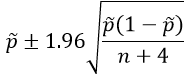
The p-tilde symbol here represents the modified sample proportion, after including the fictional successes and failures.  In other words, if x represents the number of successes, then p-tilde = (x + 2) / (n + 4). 

How does p-tilde compare to p-hat?  Often a student will say that p-tilde is larger than p-hat, or smaller than p-hat.  Then I respond with a hint: What if p-hat is less than 0.5, or equal to 0.5, or greater than 0.5?  At this point, some students realize that p-tilde is closer to 0.5 than p-hat, or equal to 0.5 if p-hat was already equal to 0.5.

Does this fairly simple plus-four adjustment really fix the problem?  Let’s find out with … simulation!  Here are the results for the same 500 simulated samples that we looked at above:

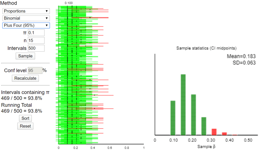
Sure enough, this plus-four method generated a 93.8% success rate among these 500 intervals.  In the long run (with this case of n = 15 and π = 0.1), the success rate approaches 94.4%.  This is very close to the nominal confidence level of 95%, vastly better than the 79.2% success rate with the conventional (Wald) method.  The graph of the distribution of 500 simulated p-tilde values on the right above reveals the cause for the improvement: The plus-four procedure now succeeds when there are 0 successes in the sample, producing a p-tilde value of 2/19 ≈ 0.105, and this procedure fails only with 4 or more successes in the sample.

Because of the discrete-ness of a binomial distribution with a small sample size, the coverage probability is very sensitive to small changes.  For example, increasing the sample size from n = 15 to n = 16, with a population proportion of π = 0.1, increases the coverage rate with the 95% plus-four procedure from 94.4% to 98.3%.  Having a larger coverage rate than the nominal confidence level is better than having a smaller one, but notice that the n = 16 rate misses the target value of 95% by more than the n = 15 case.  Still, the plus-four method produces a coverage rate much closer to the nominal confidence level than the conventional method for all small sample sizes.

Let’s practice applying this plus-four method to sample data from the blindsight study that I described in post #12 (Simulation-based inference, part 1, here).  A patient who suffered brain damage that caused vision loss on the left side of her visual field was shown 17 pairs of house drawings.  For each pair, one of the houses was shown with flames coming out of the left side.  The woman said that the houses looked identical for all 17 pairs.  But when she was asked which house she would prefer to live in, she selected the non-burning house in 14 of the 17 pairs.

The population proportion π to be estimated here is the long-run proportion of pairs for which the patient would select the non-burning house, if she were to be shown these pairs over and over.  Is the sample size condition for the conventional (Wald) confidence interval procedure satisfied?  No, because the sample consists of only 3 “failures,” which is considerably less than 10.  Calculate the point estimate for the plus-four procedure.  We pretend that the sample consisted of two additional “successes” and two additional “failures.”  This gives us p-tilde = (14 + 2) / (17 + 4) = 16/21 ≈ 0.762.  How does this compare to the sample proportion?  The sample proportion (of pairs for which she chose the non-burning house) is p-hat = 14/17 ≈0.824.  The plus-four estimate is smaller, as it is closer to one-half.  Use the plus-four method to determine a 95% confidence interval for the population proportion.  This confidence interval is: 0.762 ± 1.96×sqrt(0.762×0.238/21), which is 0.762 ± 0.182, which is the interval (0.580 → 0.944).  Interpret this interval.  We can be 95% that in the long run, the patient would identify the non-burning house for between 58.0% and 94.4% of all showings.  This interval lies entirely above 0.5, so the data provide strong evidence that the patient does better than randomly guessing between the two drawings.  Why is this interval so wide?  The very small sample size, even after adding four hypothetical responses, accounts for the wide interval.  Is this interval valid, despite the small sample size?  Yes, the plus-four procedure compensates for the small sample size.

---

We have tackled three different “what would go wrong if a condition was not satisfied?” questions and found the same answer every time: A (nominal) 95% confidence interval would succeed in capturing the actual parameter value less than 95% of the time, sometimes considerably less.  I trust that this realization helps to dispel the conspiracy theory among students that we introduce such complications only to torment them.  On the contrary, our goal is to use procedures that actually succeed 95% of the time when that’s how often they claim to succeed.

As a wrap-up question for students on this topic, I suggest asking once again: What does the word “succeed” mean when we speak of a confidence interval procedure succeeding 95% of the time?  I hope they realize that “succeed” here means that the interval includes the actual (but unknown in real life, as opposed to a simulation) value of the population parameter.  I frequently remind students to think about the green intervals, as opposed to the red ones, produced by the applet simulation, and I ask them to remind me how the applet decided whether to color the interval as green or red.