#28 A pervasive pet peeve

Let’s suppose that you and I are both preparing to teach our next class.  Being easily distracted, I let my mind (and internet browser) wander to check on my fantasy sports teams, so I only devote 60% of my attention to my class preparation.  On the other hand, you keep distractions to a minimum and devote 90% of your attention to the task.  Let’s call these values (60% for me, 90% for you) our focus percentages.  Here’s the question on which this entire post hinges: Is your focus percentage 30% higher than mine?

I have no doubt that most students would answer yes.  But that’s incorrect, because 90 is 50% (not 30%) larger than 60.  This mistaking of a difference in percentages as a percentage difference is the pet peeve that permeates this post.

I will describe some class examples that help students learn how to work with percentage differences.  Then I’ll present some assessment items for giving students practice with this tricky idea.  Along the way I’ll sneak in a statistic that rarely appears in Stat 101 courses: relative risk.  As always, questions for students appear in italics.

---

A rich source of data on high school students in the United States is the Youth Risk Behavior Surveillance Survey (YRBSS).  Here are counts from the 2017 YRBSS report, comparing youths in Arizona and California on how often they wear a seat belt when riding in a car driven by someone else:

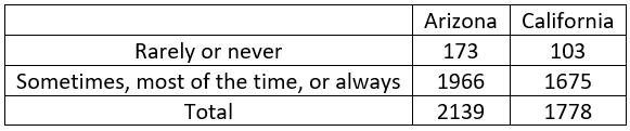
For each state, calculate the proportion (to three decimal places) of respondents who rarely or never wear a seat belt.  These proportions are 173/2139 ≈ 0.081 for Arizona, 103/1778 ≈ 0.058 for California.  Convert these proportions to percentages, and use these percentages in sentences*.  Among those who were surveyed, 8.1% of the Arizona youths and 5.8% of the California youths said that they rarely or never wear a seat belt when riding in a car driven by someone else.

* I think it’s worthwhile to explicitly ask students to convert proportions to percentages.  It’s more common to speak about percentages than proportions, and this conversion is non-trivial for some students.

Is it correct to say that Arizona youths in the sample were 2.3% more likely to wear a seat belt rarely or never than California youths in the sample?  Some students need a moment to press 8.1 – 5.8 into their calculator or cell phone to confirm the value 2.3, and then almost all students respond yes.

Let me pause here, because I want to be very clear: This is my pet peeve.  I explain that the difference between the two states’ percentages (8.1% and 5.8%) is 2.3 percentage points, but that’s not the same thing as a 2.3 percent difference.

---

At this point I ask students to indulge me in a brief detour.  Percentage difference between any two values is often tricky for people to understand, but working with percentages as the two values to be compared makes the calculation and interpretation all the more confusing. The upcoming detour simplifies this by using more generic values than percentages.

Suppose that my IQ is 100* and Beth’s is 140.  These IQ scores differ by 40 points.  What is the percentage difference in these IQ scores?  I quickly admit to my students that this question is not as clear as it could be.  When we talk about percentage difference, we need to specify compared to what.  In other words, we need to make clear which value is the reference (or baseline).  Let me rephrase: By what percentage does Beth’s IQ exceed mine?  Now we know that we are to treat my IQ score as the reference value, so we divide the difference by my IQ score: (140 – 100) / 100 = 0.40.  Then to express this as a percentage, we multiply by 100% to obtain: 0.40×100% = 40%.  There’s our answer: Beth’s IQ score is 40% larger than mine.

* I joked about my IQ score in post #5, titled A below-average joke, here.

Why did this percentage difference turn out to be the same as the actual difference?  Because the reference value was 100, and percent means out of 100.  Let’s make the calculation slightly harder by bringing in Tom, whose IQ is 120.  By what percentage does Beth’s IQ exceed Tom’s?  Using Tom’s IQ score as the reference gives a percentage difference of: (140 – 120) / 120 × 100% ≈ 16.7%.  Beth’s IQ score, which is 20 points higher than Tom’s, is 16.7% greater than Tom’s.

Does this mean that Tom’s IQ score is 16.7% below Beth’s?  Many students realize that the answer is no, because this question changes the reference value to be Beth’s rather than Tom’s.  The calculation is now: (120 – 140) / 140 × 100% ≈ -14.3%.  Tom’s IQ score is 14.3% lower than Beth’s.

Calculate and interpret the percentage difference between Tom’s IQ score and mine, in both directions.  Comparing Tom’s IQ score to mine is the easier one, because we’ve seen that a reference value of 100 makes calculations easier: (120 – 100) / 100 × 100% ≈ 20%.  Tom’s IQ score is 20% higher than mine.  Comparing my score to Tom’s gives: (100 – 120) / 120 × 100% ≈ -16.7%.  My IQ score is 16.7% lower than Tom’s*.

* I think I can hear what many of you are thinking: Wait a minute, this is not statistics!  I agree, but I nevertheless think this topic, which should perhaps be classified as numeracy, is relevant and important to teach in introductory statistics courses.  Otherwise, many students will continue to make mistakes throughout their professional and personal lives when working with and interpreting percentages.  I will end this detour and return to examining real data now.

Let’s return to the YRBSS data.  Calculating a percentage difference can seem more complicated when dealing with proportions, but the process is the same.  Calculate the percentage difference by which the Arizona youths’ proportion who rarely or never use a seat belt exceeds that for California youths.  Earlier we calculated the difference in proportions to be: 0.081 – 0.058 = 0.023. Now we divide by California’s baseline value to obtain: 0.023/0.058 ≈ .396, and finally we convert this to a percentage difference by taking: 0.396 × 100% = 39.6%.  Write a sentence interpreting this value in context.  Arizona youths in this sample were 39.6% more likely to rarely or never wear a seat belt than California youths.  Finally, just to make sure that my pet peeve is not lost on students: Is this percentage difference of 39.6% close to the absolute difference of 2.3 percentage points?  Not at all!

---

Next I take students on what appears to be a tangent but will lead to a connection with a different statistic for comparing proportions between two groups.  Calculate the ratio of proportions who rarely or never use a seat belt between Arizona and California youths in the survey.  This calculation is straightforward: 0.081/0.058 ≈ 1.396.  Write a sentence interpreting this value in context.  Arizona youths in the survey are 1.396 times more likely to rarely or never wear a seat belt than California youths.  I emphasize that the word times is a crucial one in this sentence.  The word times is correct here because we calculated a ratio in the first place.

Then I reveal to students that this new statistic (ratio of proportions) is important enough to have its own name: relative risk.  The relative risk of rarely or never wearing a seat belt, comparing Arizona to California youths, is 1.396.  The negative word risk is used here because this statistic is often reported in medical studies, comparing proportions with a negative result such as having a disease.  The convention is to put the larger proportion in the numerator, using the smaller proportion to indicate the reference group.

Does the number 1.396 look familiar from our earlier analysis?  Most students respond that the percentage difference was 0.396, which seems too strikingly similar to 1.396 to be a coincidence.  Make a conjecture for the relationship between percentage difference and relative risk.  Many students propose: percentage difference = (relative risk – 1) × 100%.

I ask students to test this conjecture with YRBSS data on seat belt use from Pennsylvania and California youths:

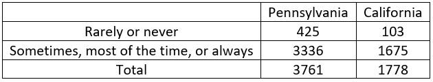
Calculate and interpret the difference and ratio of proportions who rarely or never use seat belts.  The “rarely or never” proportion in Pennsylvania is 425/3761 ≈ 0.113.  We’ve already calculated that the proportion in California is 103/1778 ≈ 0.058.  The difference in proportions is 0.113 – 0.058 = 0.055.  The percentage of Pennsylvania youths in the sample who said that they rarely or never wear a seat belt is 5.5 percentage points higher than the percentage of California youths who answered “rarely or never.”  The ratio of proportions is 0.113/0.058 ≈ 1.951*.  A Pennsylvania youth in the sample was 1.951 times more likely than a California youth to rarely or never wear a seat belt.

* I performed this calculation on the actual counts, not the proportions rounded to three decimal places in the numerator and denominator.

Verify that the conjectured relationship between percentage difference and relative risk holds.  The percentage difference in the proportions can be calculated as: (0.113 – 0.058) / 0.058 × 100% ≈ 95.1%.  This can also be calculated from the ratio as: (1.951 – 1) × 100% ≈ 95.1%.

I am not necessarily proposing that relative risk needs to be taught in Stat 101 courses.  I am urging a very careful treatment of percentage difference, and it takes just an extra 15 minutes of class time to introduce relative risk.

---

Let’s follow up with a confidence interval for a difference in proportions.  If we go back to comparing the responses from Arizona and California youths, a 95% confidence interval for the difference in population proportions turns out to be: .023 ± .016, which is the interval (.007 → .039).

Interpret what this interval reveals.  First recall that the order of subtraction is Arizona minus California, and notice that the interval contains only positive values.  We are 95% confident that the proportion of all Arizona youths who would answer that they rarely or never wear a seat belt is between .007 and .039 larger than the proportion of all California who would give that answer.  We can translate this answer to percentage points by saying that the Arizona percentage (of all youths who would answer that they rarely or never wear a seat belt) is between 0.7 and 3.9 percentage points larger than the California percentage.  But many students trip themselves up by saying that Arizona youths are between 0.7% and 3.9% more likely than California youths to answer that they rarely or never wear a seat belt.  This response is incorrect, for it succumbs to my pet peeve of mistakenly interpreting a difference in percentages as a percentage difference.

What parameter do we need to determine a confidence interval for, in order to estimate the percentage difference in population proportions (who rarely or never wear a seat belt) between Arizona and California youths?  A confidence interval for the population relative risk will allow this.  Such a procedure exists, but it is typically not taught in an introductory statistics course*.  For the YRBBS data on seat belt use in Arizona and California, a 95% confidence interval for the population relative risk turns out to be (1.103 → 1.767).

* The sampling distribution of a sample relative risk is skewed to the right, but the sampling distribution of the log transformation of the sample relative risk is approximately normal.  So, a confidence interval can be determined for the log of the population relative risk, which can then be transformed back to a confidence interval for the population relative risk.

What aspect of this interval indicates strong evidence that Arizona and California have different population proportions?  This can be a challenging question for students, so I often offer a hint: What value would the relative risk have if the two population proportions were the same?  Most students realize that the relative risk (ratio of proportions) would equal 1 in this case.  That the interval above is entirely above 1 indicates strong evidence that Arizona’s population proportion (who rarely or never wear a seat belt) is larger than California’s.

Interpret this confidence interval.  We are 95% confident that Arizona youths are between 1.103 and 1.767 times more likely than California youths to answer that they rarely or never wear a seat belt.  Convert this to a statement about the percentage difference in the population proportions.  We can convert this to percentage difference by saying: We are 95% confident that Arizona youths are between 10.3% and 76.7% more likely than California youths to answer that they rarely or never wear a seat belt.

I am not suggesting that students learn how to calculate a confidence interval for a relative risk in Stat 101, but I do think students should be able to interpret such a confidence interval.

---

Now we return to the YRBSS data for a comparison that illustrates another difficulty that some students have with percentages.  The YRBSS classifies respondents by race, and the 2017 report says that 9.8% of black youths and 4.3% of white youths responded that they rarely or never wear a seat belt.  Calculate the ratio of these percentages.  This ratio is: .098/.043 ≈ 2.28.  Write a sentence interpreting the relative risk.  Black youths who were surveyed were 2.28 times more likely than white youths to rarely or never wear a seat belt.  Complete this sentence: Compared to white youths who were surveyed, black youths were ______ % more likely to rarely or never wear seat belts.  To calculate the percentage difference, we can use the relative risk as we discovered above: (2.28 – 1) × 100% = 128%.  Black youths who were surveyed were 128% more likely to rarely or never wear seat belts, as compared to white youths.

Hold on, can a percentage really be larger than 100%?  Yes, a percentage difference (or a percentage change or a percentage error) can exceed 100%.  If one value is exactly twice as big as another, then it is 100% larger.  So, if one value is more than twice as big as another, then it is more than 100% larger.  In this case, the percentage (who rarely or never use a seat belt) for black youths is more than twice the percentage for white youths, so the relative risk exceeds 2, and the percentage difference between the two percentages therefore exceeds 100%.

---

Here is a quiz containing five questions, all based on real data, for giving students practice working with percentage differences:

• a) California’s state sales tax rate in early 2019 was 7.3%, compared to Hawaii’s state sales tax rate of 4.0%.  Was California’s state sales tax rate 3.3% higher than Hawaii’s?  If not, determine the correct percentage difference to use in that sentence.
• b) Alaska had a 0% state sales tax rate in early 2019.  Could Hawaii match Alaska’s rate by reducing theirs by 4%?  If not, determine the correct percentage reduction to use in that sentence.
• c) Steph Curry successfully made 354 of his 810 (43.7%) three-point shots in the 2018-19 NBA season, and Russell Westbrook successfully made 119 of his 411 (29.0%) three-point shots.  Could Westbrook have matched Curry’s success rate with a 14.7% improvement in his own success rate?  If not, determine the correct percentage improvement to use in that sentence.
• d) Harvard University accepted 4.5% of its freshman applicants for Fall 2019, and Duke University accepted 7.4% of its applicants.  Was Harvard’s acceptance rate 2.9% lower than Duke’s?  If not, then determine the correct percentage difference to use in that sentence.
• e) According to the World Bank Development Research Group, 10.0% of the world’s population lived in extreme poverty in 2015, compared to 35.9% in 1990.  Did the percentage who lived in extreme poverty decrease by 25.9% in this 25-year period?  If not, determine the correct percentage decrease to use in that sentence.

The correct answer to all of these yes/no questions is no, not even close.  Correct percentage differences are: a) 82.5% b) 100% c) 50.9% d) 39.2% e) 72.1%.

---

I briefly considered titling this post: A persnickety post that preaches about a pervasive, persistent, and pernicious pet peeve concerning percentages.  That title contains 15 words, 9 of which start with the letter P, so 60% of the words in that title begin with P.  Instead I opted for the much simpler title: A pervasive pet peeve, for which 75% of the words begin with P. 

Does this mean that I increased the percentage of P-words by 15% when I decided for the shorter title?  Not at all, that’s the whole point!  I increased the percentage of P-words by 15 percentage points, but that’s not the same as 15%.  In fact, the percentage increase is (75 – 60) / 60 × 100% = 25%, not 15%. 

Furthermore, notice that 25% is 66.67% larger than 15%, so the percentage increase (in percentage of P-words) that I achieved with the shorter title is 66.67% greater than what many would mistakenly believe the percentage increase to have been.

No doubt I have gotten carried away*, as that last paragraph is correct but positively** ridiculous.  I’ll conclude with two points: 1) Misunderstanding percentage difference (or change) is very common, and 2) Teachers of statistics can help students to calculate and interpret percentage difference correctly.

* You might have come to that conclusion far earlier in this post.

** I couldn’t resist using another P word here. I really need to press pause on this preposterous proclivity.

P.S. The 2017 YRBSS report can be found here.  You might ask students to select their own questions and variables to analyze and compare. Data on state sales tax rates appear here, basketball players’ shooting percentages here, college acceptance rates here, and poverty rates here.