#12 Simulation-based inference, part 1

We have had tastes of simulation-based inference (abbreviated SBI) in earlier posts.  Post #2 (here), about my all-time favorite question, presented simulation results for the statistic (mean/median) as a measure of skewness.  Post #9 (here), about the 1970 draft lottery, presented a simulation analysis of the correlation coefficient as a measure of lottery fairness.  Now let’s take a step back and consider how one might first introduce students to the concept of statistical inference, more specifically the concept of strength of evidence, through simulation.  You could do this near the very beginning of a course as an introduction to statistical thinking, or you could present this as an introduction to a unit on statistical inference.

Let’s start with real data from a genuine research study in brain science* (described here).  A patient suffered brain damage that caused a loss of vision on the left side of her visual field.  A researcher showed two cards to this patient.  Each card showed a simple line drawing of a house.  However, one of the drawings showed flames coming out of the left side of the house.  The researcher shuffled the two cards, placed them down on a table with one card above the other, and asked the patient which house she would rather live in.  The patient replied that this was a silly question because “they are the same.”  The researcher asked her to choose anyway. The cards were shuffled and placed on the table a total of 17 times. The patient chose the non-burning house in 14 of those 17 showings.  The researcher investigated whether these data provide strong evidence that this patient has a condition known as “blindsight,” meaning that she responds to information from the blind part of her visual field even though she cannot “see” those stimuli.

* I learned about this study from a presentation by Rob Kass at the 2017 U.S. Conference on Teaching Statistics, and I saw Doug Tyson give a workshop presentation about using this context to introduce simulation-based inference.

After I present the background of this study, I first ask students*: Identify the observational units and variable in this study.  The observational units are the 17 showings of pairs of cards, and the variable is which house the patient chose, a binary categorical variable.  Then I ask an obvious question: Did the patient identify the non-burning house for more than half of the showings?  Of course the answer is yes, but I think this question helps to prepare students for the challenging question that comes next: Identify two possible explanations for this result.

* Those of you who read post #11 (here) will not be surprised by this.

I often have to nudge students in the direction I’m looking for.  I have in mind that one explanation is that this patient truly has blindsight, so she really is more likely to choose the non-burning house.  The other explanation, which is surprisingly difficult for students to consider without prompting, is that the patient’s selections are simply the result of random chance. In other words, this second explanation asserts that the patient is equally likely to choose either version of the house on each showing.

Then I ask: Which of these two explanations is easier to investigate, and how might we investigate it with a common device?  Most students realize that the “random chance” explanation is fairly easy to investigate by tossing a coin.  How many coin tosses do we need?  Seventeen, one for each showing of a pair of houses to the patient.  What will heads and tails represent?  Heads will represent choosing the non-burning house, tails will represent choosing the burning house.  (Or you could swap these, it doesn’t matter which is which.)

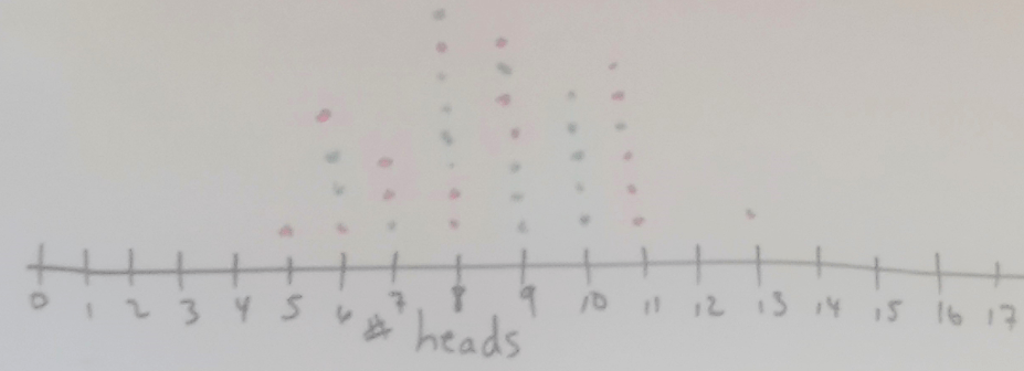
At this point I ask each student in the class to toss a coin* 17 times and count the number of heads.  As the students finish their tosses, they go to the board and put a dot on a dotplot to indicate how many heads they obtained in their 17 tosses.  In this manner a class of 35 students produces a graph** such as:

* I recommend taking coins to class with you, because carrying coins is not very common for today’s students!

** You might ask students about the observational units and variable in this graph.  The variable is fairly clear and should appear in the axis label: number of heads in 17 coin tosses.  But the observational units are trickier to think about: 35 sets of 17 coin tosses.  I often wait until the end of the activity to ask students about this, because I don’t want to distract attention from the focus on understanding strength of evidence.

What can we learn from this graph, about whether the study’s result provides strong evidence that this patient has blindsight?  The important aspect of the graph for addressing this question is not the symmetric shape or the center near 8.5 (half of 17), although those are worth pointing out as what we expect in this situation.  Our goal is to assess whether the observed result for this patient (14 selections of the non-burning house in 17 showings) would be surprising, if in fact the subject’s selections were random.  What’s important in the graph is that none of these 35 repetitions of the study produced 14 or more heads in 17 simulated coin tosses.  This suggests that it would be pretty surprising to obtain a result as extreme as the one in this study, if the subject was making selections at random.  So, this suggests that the patient’s selections were not random, that she was actually more likely to select the non-burning house.  In other words, our simulation analysis appears to provide fairly strong evidence that this subject truly has blindsight.

Now I hope that a student will ask: Wait a minute, is 35 repetitions enough to be very informative?  Good question! We really should conduct this simulation analysis with thousands of repetitions, not just 35, in order to get a better sense for what would happen if the subject’s selections are random.  I jokingly ask students whether they would like to spend the next several hours tossing coins, but we agree that using software would be much quicker.

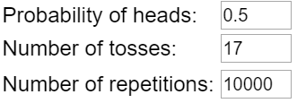
We turn to an applet from the RossmanChance* collection to perform the simulation (link; click on One Proportion).  First we need to provide three inputs for the simulation analysis:

* As I have mentioned before, Beth Chance deserves virtually all of the credit for these applets.

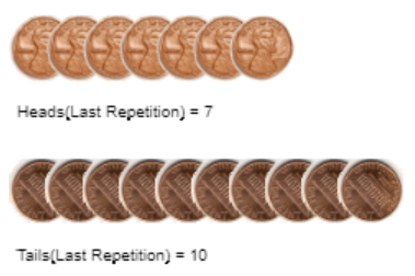
One of my favorite aspects of this applet is that it mimics the tactile simulation.  The applet shows coins being tossed, just as students have already done with their own coins:

Here are the results of 10,000 repetitions:

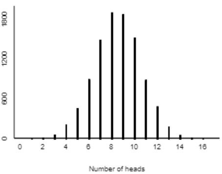
With so many repetitions, we now have a very good sense for what would happen with 17 selections made at random, if this study were repeated over and over.  We see a symmetric distribution centered around 8.5 heads.  We also notice that getting 14 heads in 17 tosses is not impossible with a random coin.  But we see (and this is the key) that it’s very unlikely to obtain 14 or more heads in 17 tosses of a random coin.  We can take this one step further by counting how many of the 10,000 repetitions produced 14 or more heads:

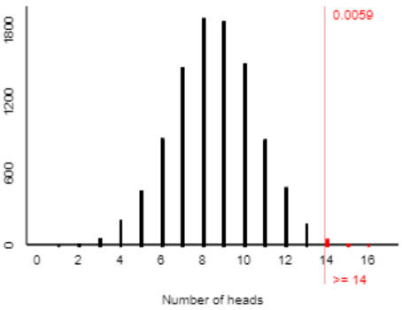
In 10,000 simulated repetitions of this study, under the assumption that only random chance controlled the patient’s selections, we find that only 59 of those repetitions (less than one percent) resulted in 14 or more selections of the non-burning house.  What can we conclude from this, and why?  Well, this particular patient really did select the non-burning house 14 times.  That would be a very surprising result if she were making selections randomly.  Therefore, we have very strong evidence that the patient was not making selections randomly, in other words that she does have this ability known as blindsight.

There you have it: the reasoning process of statistical inference as it relates to strength of evidence, presented in the context of real data from a genuine research study.  I think students can begin to grasp that reasoning process after a half-hour activity such as this.  I think it’s important not to clutter up the presentation with unnecessary terminology and formalism.  Some of the most important decisions a teacher makes concern what to leave out.  We have left out a lot here: We have not used the terms null and alternative hypothesis, we have not identified a parameter, we have not calculated a test statistic, we have not used the term p-value, we have not spoken of a test decision or significance level or rejecting a null hypothesis.  All of that can wait for future classes; keep the focus for now on the underlying concepts and reasoning process.

Before the end of this class period, I like to introduce students to a new study to see whether they can reproduce such a simulation analysis, draw the appropriate conclusion about strength of evidence, and explain the reasoning process behind their conclusion.  Here’s a fun in-class data collection, based again on a genuine research study: A phenomenon called facial prototyping suggests that people tend to associate certain facial characteristics with certain names.  I present students with two faces from the article here), tell them that the names are Bob and Tim, and ask who (Bob or Tim) is on the left:

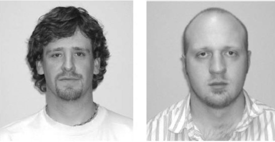
In a recent class, 36 of 46 students associated the name Tim with the face on the left.  I asked my students: Conduct a simulation analysis to investigate whether this provides strong evidence that college students have a tendency to associate Tim with the face on the left.  Summarize your conclusion, and explain your reasoning.

First students need to think about what values to enter for the applet inputs:

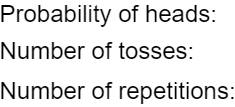
Just as with the blindsight study, we again need 0.5 for the probability of heads, because if people attach names to faces at random, they would put Tim on the left 50% of the time.  We need 46 tosses, one for each student in the sample.  Any large number will suffice for the number of repetitions; I like to use 10,000. Here are the results:

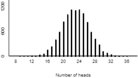
We see that it’s incredibly unlikely to obtain 36 or more heads in 46 tosses of a random coin.  So, it would be extremely surprising for 36 or more of 46 students to attach Tim to the face on the left, if in fact students make selections purely at random.  Therefore, our class data provide very strong evidence that college students do have a genuine tendency to associate the name Tim with the face on the left.

I like starting with the blindsight example before facial prototyping, because I find it comforting to know in advance that the data are 14 successes in 17 trials for the first example.  I also like that the p-value* turns out to be less than .01 in the blindsight example.  Collecting data from students in class is fun and worthwhile, but you never know in advance how the data will turn out.  The Bob/Tim example is quite dependable; I have used it with many classes and have found consistent results that roughly 65-85% put Tim on the left.

* I’m very glad to be able to use this term with you, even though I hold off on using it with my students.  Having a common language that your readers understand can save a lot of time!

Simulation-based inference (SBI) has become a prominent aspect of my teaching, so it will be a common theme throughout this blog.  Part 2 of this post will introduce SBI for comparing two groups, but I will hold off on that post for a while.  Next week’s post will continue the SBI theme by asking which you put more trust in: simulation-based inference or normal-based inference?

P.S. Simulation-based inference has become much more common in introductory statistics textbooks over the past decade.  One of the first textbooks to put SBI front-and-center was Statistics: Learning in the Presence of Variation, by Bob Wardrop.  I consider Wardrop’s book, published in 1993, to have been ahead of its time.  Beth Chance and I focused on SBI in Investigating Statistical Concepts, Applications, and Methods (ISCAM), which is an introductory textbook aimed at mathematically inclined students (link).  Intended for a more general audience, Introduction to Statistical Investigations presents SBI beginning in chapter 1.  I contributed to this textbook, written by an author team led by Nathan Tintle (link) and making use of Beth’s applets (link). The Lock family has written a textbook called Statistics: Unlocking the Power of Data in which SBI figures prominently (link), using StatKey software (link).  Josh Tabor and Chris Franklin have written Statistical Reasoning in Sports, which uses SBI extensively (link) and has an accompanying collection of applets (link). Andy Zieffler and the Catalysts for Change group at the University of Minnesota have also developed a course and textbook for teaching statistical thinking with SBI (link), making use of TinkerPlots software (link). This list is by no means exhaustive, and instructors can certainly use other software tools, such as R, to implement SBI.  Dozens of instructors have contributed advice to a blog about teaching SBI (link).