#10 My favorite theorem

This blog does not do suspense*, so I’ll come right out with it: Bayes’ Theorem is my favorite theorem.  But even though it is my unabashed favorite, I introduce Bayes’ Theorem to students in a stealth manner.  I don’t present the theorem itself, or even its name, until after students have answered an important question by essentially deriving the result for themselves.  The key is to use a hypothetical table of counts, as the following examples illustrate.  As always, questions that I pose to students appear in italics.

* See question #8 in post #1 here.

1. The ELISA test for HIV was developed in the mid-1980s for screening blood donations.  An article from 1987 (here) gave the following estimates about the ELISA test’s effectiveness in the early stages of its development:

• The test gives a (correct) positive result for 97.7% of blood samples that are infected with HIV.
• The test gives a (correct) negative result for 92.6% of blood samples that are not infected with HIV.
• About 0.5% of the American public was infected with HIV.

First I ask students: Make a prediction for the percentage of blood samples with positive test results that are actually infected with HIV.  Very few people make a good prediction here, but I think this prediction step is crucial for creating cognitive dissonance that leads students to take a closer look at what’s going on.  Lately I have rephrased this question as multiple choice, asking students to select whether their prediction is closest to 10%, 30%, 50%, 70%, or 90%.  Most students respond with 70% or 90%.

Then I propose the following solution strategy: Assume that the given percentages hold exactly for a hypothetical population of 1,000,000 people, and use the percentages fill in the following table of counts:

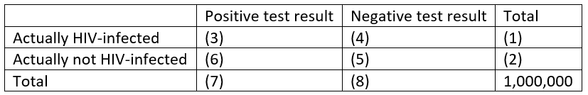
The numbers in parentheses indicate the order in which we can use the given percentages to complete the table of counts.  I insist that all of my students get out their calculators, or use their phone as a calculator, as we fill in the table together, as follows:

1. 005 × 1,000,000 = 5,000
2. 1,000,000 – 5,000 = 995,000
3. 0.977 × 5,000 = 4,885
4. 5,000 – 4,885 = 115
5. 0.926 × 995,000 = 921,370
6. 995,000 – 921,370 = 73,630
7. 4,885 + 73,630 = 78,515
8. 115 + 921,370 = 921,485

These calculations produce the following table:

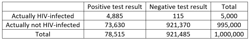
Then I say to my students: That was fun, and it filled 10 minutes of class time, but what was the point?  What do we do now with this table to answer the original question?  Many students are quick to point out that we can determine the percentage of positive results that are actually HIV-infected by starting with 78,515 (the total number of positive results) as the denominator and using 4,885 (the number of these positive results that are actually HIV-infected) as the numerator.  This produces: 4,885 / 78,515 ≈ 0.062, or 6.2%.

At this point I act perplexed* and say: Can this really be right?  Why would this percentage be so small when the accuracy percentages for the test are both greater than 90%?  This question is much harder for students, but I encourage them to examine the table and see what’s going on.  A student eventually points out that there are a lot more false positives (people who test positive but do not have the disease) than there are true positives (people who test positive and do have the disease).  Exactly! And why is that?  I often need to direct students’ attention to the base rate: Only half of one percent have the disease, so a very large percentage of them are outnumbered by a fairly small percentage of the 99.5% who don’t have the disease.  In other words, 7.4% of 995,000 people greatly outnumbers 97.7% of 5,000 people.

* I am often truly perplexed, so I have no trouble with acting perplexed to emphasize a point.

I like to think that most students understand this explanation, but there’s no denying that this is a difficult concept.  Simply understanding the question, which requires recognizing the difference between the two conditional percentages (percentage of people with disease who test positive versus percentage of people with positive test result who have disease), can be a hurdle.  To help with this I like to ask: What percentage of U.S. Senators are American males?  What percentage of American males are U.S. Senators?  Are these two percentages the same, fairly close, or very different?  The answer to the first question is a very large percentage: 80/100 = 80% in 2019, but the answer to the second question is an extremely small percentage: 80 / about 160 million ≈ 0.00005%.  These percentages are very different, so it shouldn’t be so surprising that the two conditional percentages* with the ELISA test are also quite different.  At any rate I am convinced that the table of counts makes this more understandable than plugging values into a formula for Bayes’ Theorem would.

* I have avoided using the term conditional probability here, because I think the term conditional percentage is less intimidating to students, suggesting something that can be figured out from a table of counts rather than requiring a mathematical formula.

Some students think this fairly small percentage of 6.2% means that the test result is not very informative, so I ask: How many times more likely is a person to be HIV-infected if they have tested positive, as compared to a person who has not been tested?  This requires some thought, but students recognize that they need to compare 6.2% with 0.5%.  The wording how many times can trip some students up, but many realize that they must take the ratio of the two percentages: 6.2% / 0.5% = 12.4. Then I challenge students with: Write a sentence, using this context, to interpret this value.  A person with a positive test result is 12.4 times more likely to be HIV-infected than someone who has not yet been tested.

I also ask students: Can a person who tests negative feel very confident that they are free of the disease?  Among the blood samples that test negative, what percentage are truly not HIV-infected?  Most students realize that this answer can be determined from the table above: Among the 921,485 who test negative, 921,370 do not have the disease, which is a proportion of 0.999875, or 99.9875%.  A person who tests negative can be quite confident that they do not have the disease.  Such a very high percentage is very important for screening blood donations.  It’s less problematic that only 6.2% of the blood samples that are rejected (due to a positive test result) are actually HIV-infected.

You might want to introduce students to some terminology before moving on.  The 97.7% value is called the sensitivity of the test, and the 92.6% value is called the specificity.  You could also tell students that they have essentially derived a result called Bayes’ Theorem as they produced and analyzed the table of counts.  You could give them a formula or two for Bayes’ Theorem.  The one on the left, presented in terms of H for hypothesis and E for evidence, has a two-event partition (such as disease, not).  A more general of Bayes’ Theorem appears on the right.

I present these versions of Bayes’ Theorem in probability courses and in courses for mathematically inclined students, but I do not show any formulas in my statistical literacy course.  For a standard “Stat 101” introductory course, I do not present this topic at all, as the focus is exclusively on statistical concepts and not probability.

Before we leave this example, I remind students that these percentages were from early versions of the ELISA test in the 1980s, when the HIV/AIDS crisis was first beginning.  Improvements in testing procedures have produced much higher sensitivity and specificity (link).  Running more sophisticated tests on those who test positive initially also greatly decreases the rate of false positives.

I have debated with myself whether to change this HIV testing context for students’ first introduction to these ideas.  One argument against using this context is that the information about sensitivity and specificity is more than three decades old.  Another argument is that 97.7% and 92.6% are not convenient values to work with; perhaps students would be more comfortable with “rounder” values like 90% and 80%.  But I continue to use this context, partly to remind students of how serious the HIV/AIDS crisis was, and because I think the example is compelling.  An alternative that I found recently is to present these ideas in terms of a 2014 study of diagnostic accuracy of breathalyzers sold to the public (link).

Where to next?  With my statistical literacy course, I give students more practice with constructing and analyzing tables of counts to calculate reverse conditional percentages, as in the following example.

A national survey conducted by the Pew Research Center in late 2018 produced the following estimates about educational attainment and Twitter use among U.S. adults:

• 10% have less than a high school diploma; 8% of these adults use Twitter
• 59% have a high school diploma but no college degree; 20% of these adults use Twitter
• 31% have a college degree; 30% of these adults use Twitter

What percentage of U.S. adults who use Twitter have less than a high school diploma?  What percentage have a high school degree but no college degree?  What percentage have a college degree?Which age groups are more likely than they were initially?  Which are less likely?

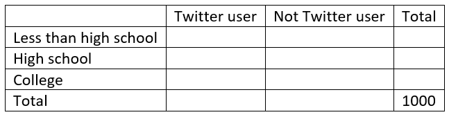
Again we can answer these questions (about reverse conditional percentages from what was given) by constructing a table of counts for a hypothetical population.  This time we need three rows rather than two, in order to account for the three education levels. I recommend providing students with the outline of the table, but without indicating the order in which to fill it in this time:

With numbers in parentheses again indicating the order in which the cells can be calculated, the completed table turns out to be:

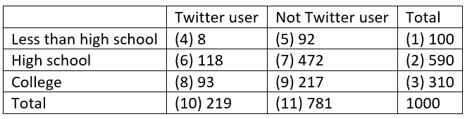
From this table we can calculate that 8/219 ≈ .037, or 3.7% of Twitter users have less than a high school degree, 118/219 ≈ .539, or 53.9% of Twitter users have a high school but not college degree, and 93/219 ≈ .425, or 42.5% of Twitter users have a college degree.  These percentages have increased from the base rate only for the college degree holders, as 31% of the public has a college degree but 42.5% of Twitter users do.

3. A third application that I like to present concerns the famous Monty Hall Problem.  Suppose that a new car is hidden behind one door on a game show, while goats are hidden behind two other doors.  A contestant picks a door, and then (to heighten the suspense!) the host reveals what’s behind a different door that he knows to have a goat.  Then the host asks whether the contestant prefers to stay with the original door or switch to the remaining door.  The question for students is: Does it matter whether the contestant stays or switches?  If so, which strategy is better, and why?

Most people believe that staying or switching does not matter.  I recommend that students play a simulated version of the game many times, with both strategies, to get a sense for how the strategies compare.  An applet that allows students to play simulated games appears here.  The following graph shows the results of 1000 simulated games with each strategy:

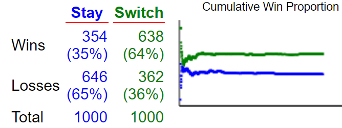
It appears that switching wins more often than staying!  We can determine the theoretical probabilities of winning with each strategy by using Bayes’ Theorem.  More to the point, we can use our strategy of constructing a table of hypothetical counts.  Let’s suppose that the contestant initially selects door #1, so the host will show a goat behind door #2 or door #3.  Let’s use 300 for the number of games in our table, just so we’ll have a number that’s divisible by 3.  Here’s the outline of the table:

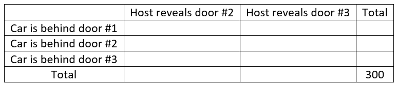
How do we fill in this table? Let’s proceed as follows:

1. Row totals: If the car is equally likely to be placed behind any of the three doors, then the car should be behind each door for 100 of the 300 games.
2. Bottom (not total) row: Remember that the contestant selected door #1, so when the car is actually behind door #3, the host has no choice but to reveal door #2 all 100 times.
3. Middle row: Just as with the bottom row, now the host has no choice but to reveal door #3 all 100 times.
4. Top row: When the car is actually behind the same door that the contestant selected, the host can reveal either of the other doors, so let’s assume that he reveals each 50% of the time, or 50 times in 100 games.

The completed table is therefore:

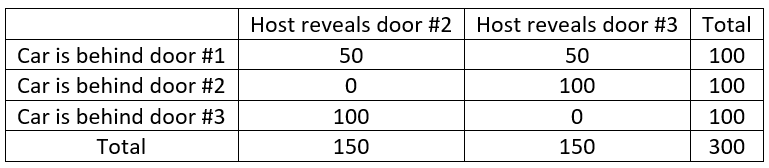
We can see from the table that for the 150 games where the host reveals door #2, the car is actually behind door #3 for 100 of those 150 games, which is 2/3 of the games.  In other words, if the contestant stays with door #1, they will win 50/150 times, but by switching to door #3, they win 100/150 times. Equivalently, for the 150 games where the host reveals door #3, the car is actually behind door #2 for 100 of those games, which is again 2/3 of the games.  Bottom line: Switching gives the contestant a 2/3 chance of winning the car, whereas staying only gives a 1/3 chance of winning the car.  The easiest way to understand this, I think, is that by switching, the contestant only loses if they picked the correct door to begin with, which happens one-third of the time.

This post is already quite long, but I can’t resist suggesting a follow-up question for students: Now suppose that the game show producers place the car behind door #1 50% of the time, door #2 40% of the time, and door #3 10% of the time.  What strategy should you use?  In other words, which door should you pick to begin, and then should you stay or switch?  What is your probability of winning the car with the optimal strategy in this case?  Explain.

Encourage students to remember the bottom line from above: By switching, you only lose if you were right to begin with.  So, the optimal strategy here is to select door #3, the least likely door, and then switch after the host reveals a door with a goat.  Then you only lose if you were right to begin with, so you only lose 10% of the time.  This optimal strategy gives you a 90% chance of winning the car.  Students who can think this through and describe the correct optimal strategy have truly understood the resolution of the famous Monty Hall Problem.

One final question for this post: Why is Bayes’ Theorem my favorite?  It provides the mechanism for updating uncertainty in light of partial information, which enables us to answer important questions, such as the reliability of medical diagnostic tests, and also fun recreational ones, such as the Monty Hall Problem.  More than that, Bayes’ Theorem provides the foundation for an entire school of thought about how to conduct statistical inference.  I’ll discuss that in a future post.

P.S. Tom Short and I wrote a JSE article (link) about this approach to teaching Bayes’ Theorem in 1995, but the idea is certainly not original with us.  Gerd Gigerenzer and his colleagues introduced the term “natural frequencies” for this approach; they have demonstrated its effectiveness for improving people’s Bayesian reasoning (link).  The Monty Hall Problem is discussed in many places, including by Jason Rosenhouse in his book (link) titled The Monty Hall Problem.  While I’m mentioning books, I will also point out Sharon Bertsch McGrayne’s wonderful book about Bayesian statistics (link), titled The Theory That Would Not Die.