#51 Randomness is hard
I enjoy three-word sentences, such as: Ask good questions. I like cats*. What about lunch**? Here’s another one: Randomness is hard.
* See post #16 (Questions about cats, here).
** I borrowed this one from Winnie-the-Pooh (see here).
What do I mean when I say that randomness is hard? I mean several things: Randomness is hard to work with, hard to achieve, hard to study. For the purpose of this post, I mean primarily that randomness is hard to predict, and also that it’s hard to appreciate just how hard randomness is to understand.
Psychologists have studied people’s misconceptions about randomness for decades, and I find these studies fascinating. I try not to overuse class examples that emphasize misunderstandings, but I do think there’s value in helping students to realize that they can’t always trust their intuition when it comes to randomness. Applying careful study and thought to the topic of randomness can be worthwhile.
In this post, I discuss some examples that reveal surprising aspects of how randomness behaves and lead students to recognize some flaws in most people’s intuition about randomness. As always, questions that I pose to students appear in italics.
I ask my students to imagine a light that flashes every few seconds. The light randomly flashes a green color with probability 0.75 and red with probability 0.25, independently from flash to flash. Then I ask: Write down a sequence of G’s (for green) and R’s (for red) to predict the colors for the next 40 flashes of this light. Before you read on, please take a minute to think about how you would generate such a sequence yourself.
Most students produce a sequence that has 30 G’s and 10 R’s, or close to those proportions, because they are trying to generate a sequence for which each outcome has a 75% chance for G and a 25% chance for R. After we discuss this tendency, I ask: Determine the probability of a correct prediction (for one of the outcomes in the sequence) with this strategy.
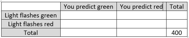
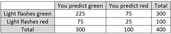
We’ll figure this out using a table of hypothetical counts*. Suppose that we make 400 predictions with this strategy. We’ll fill in the following table by assuming that the probabilities hold exactly in the table:
* For more applications of this method, see post #10 (My favorite theorem, here).
First determine the number of times that the light flashes green and the number of times that the light flashes red:
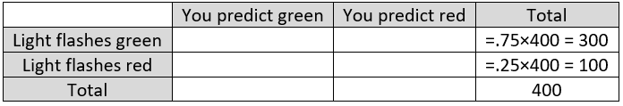
Now fill in the counts for the interior cells of the table. To do this, remember that the strategy is to predict green 75% of the time and to predict red 25% of the time, which gives:
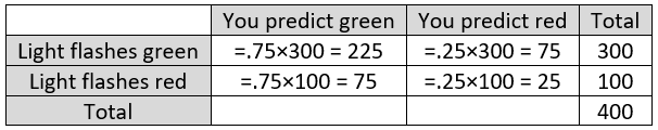
Fill in the remaining totals. This gives:
How many times is your prediction correct? You correctly predict a green light 225 times (top left cell of the table), and you correctly predict a red light 25 times (bottom right), so you are correct 250 times. These counts are shown in bold here:
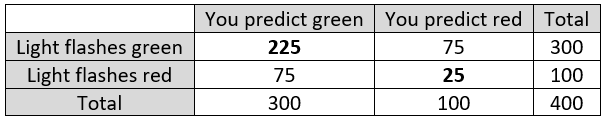
For what proportion of the 400 repetitions is your prediction correct? You are correct for 250 of the 400 repetitions, which is 250/400 = 5/8 = 0.625, or 62.5% of the time.
Here’s the key question: This is more than half the time, so that’s pretty good, right? Students are tempted to answer yes, so I have to delicately let students know that this percentage is actually, well, not so great.
Describe a method for making predictions that would be correct much more than 62.5% of the time. After a few seconds, I give a hint: Don’t overthink. And then: In fact, try a much more simple-minded approach. For students who have not yet experienced the aha moment, I offer another hint: How could you be right 75% of the time?
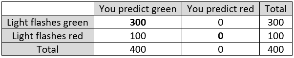
This last question prompts most students to realize that they could have just predicted green for all 40 flashes. How often will your prediction be correct with this simple-minded strategy? You’ll be correct whenever the light flashes green, which is 75% of the time. Fill in the table to analyze this strategy. The resulting table is below, with correct predictions again shown in bold. Notice that your prediction from this simple-minded strategy is correct for 300 of the 400 repetitions:
I learned of this example from Leonard Mlodinow’s book The Drunkard’s Walk: How Randomness Rules Our Lives. I recount for my students the summary that Mlodinow provides: “Humans usually try to guess the pattern, and in the process we allow ourselves to be outperformed by a rat.” Then I add: Randomness is hard*.
* At least for humans!
What percent better does the simple-minded (rat) strategy do than the guess-the-pattern (human) strategy? Well, we have determined these probabilities to be 0.750 for rats and 0.625 for humans, so some students respond that rats do 12.5% better. Of course, that’s not how percentage change works*. The correct percentage difference is [(0.750 – 0.625) / 0.625] × 100% = 20.0%. Rats do 20% better at this game than humans.
* I discussed this at length in post #28 (A persistent pet peeve, here).
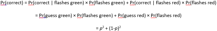
For more mathematically inclined students taking a probability course, I often ask a series of questions that generalizes this example: Now let p represent the probability that the light flashes green. Let’s stipulate that the light flashes green more often than red, so 0.5 < p < 1. The usual (human) strategy is to guess green with probability p and red with probability (1 – p). Determine the probability of guessing correctly with this strategy, as a function of p.
We could use a table of hypothetical counts again to solve this, but instead let’s directly use the law of total probability, as follows:
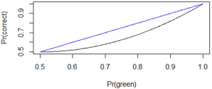
Graph this function. Here’s the graph:
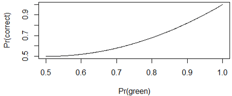
Describe the behavior of this function. This function is increasing, which makes sense, because your probability of guessing correctly increases as the lop-sidedness of the green-red breakdown increases. The function equals 0.5 when p = 0.5 and increases to 1 when p = 1. But the increase is more gradual for smaller values of p than for larger values of p, so the curve is concave up.
Determine the probability of a correct guess for our rat friends, as a function of p. This one is easy, right? Pr(correct) = p. That’s all there is to it. Rats will always guess green, so they guess correctly at whatever probability green appears.
Graph these two functions (probability of guessing correctly for humans and rats) on the same scale. Here goes, with the human graph in black and the rat graph in blue:
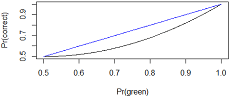
For what values of p does the rat do better (i.e., have a higher probability of success) than the human? That’s also easy: All of them!* Randomness is hard.
* Well, okay, if you want to be technical: Rats and humans tie at the extremes of p = 0.5 and p = 1.0, in case that provides any consolation for your human pride.
Where is the difference between the human and rat probabilities maximized? Examining the graph that presents both functions together, it certainly looks like the difference is maximized when p = 0.75. We can confirm this with calculus, by taking the derivative of p2 + (1-p)2 – p, setting the derivative equal to zero, and solving for p.
The “rats beat humans” example reminds me of a classic activity that asks students: Produce a sequence of 100 H’s and T’s (for Heads and Tails) that you think could represent the results of 100 flips of a fair coin.
Your prediction will be correct 50% of the time no matter how you write your sequence of Hs and Ts. This activity focuses on a different aspect of randomness, namely the consequence of the independence of the coin flips. Only after students have completed their sequence do I reveal what comes next: Determine the longest run of consecutive heads in your sequence. Then I have students construct a dotplot on the board of the distribution of their values for longest run of heads.
How can we investigate how well students performed their task of producing a sequence of coin flip outcomes? Yet again the answer I am fishing for is: Simulate! The following graph displays the resulting distribution of longest runs of heads from simulating one million repetitions of 100 flips of a fair coin:
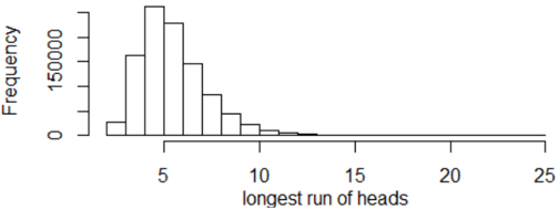
The mean of these one million results is 5.99 flips, and the standard deviation is 1.79 flips. The maximum value is 25. The proportion of repetitions that produced a longest run of 5 or more flips is 0.810, and the proportion that produced a longest run of 8 or more flips is 0.170.
How do you anticipate students’ results to differ from simulation results? Student-generated sequences almost always have a smaller mean, a smaller standard deviation, and a smaller proportion for (5 or more) and for (8 or more). Why? Because people tend to overestimate how often the coin alternates between heads and tails, so they tend to underestimate the average length for the longest consecutive run of heads. In other words, people generally do a poor job of producing a plausible sequence of heads and tails. Randomness is hard.
As a class activity, this is sometimes conducted by having half the class generate a sequence of coin flips in their head and the other half use a real coin, or a table of random digits, or a calculator, or a computer. The instructor leaves the room as both groups put a dotplot of their distributions for longest runs of heads on the board. When the instructor returns to the room, not knowing which graph is which, they can usually make a successful prediction for which is which by guessing that the student-generated graph is the one with a smaller average and less variability.
As another example that illustrates the theme of this post, I ask my students the “Linda” question made famous by cognitive psychologists Daniel Kahneman and Amos Tversky: Linda is 31 years old, single, outspoken, and very bright. She majored in philosophy. As a student, she was deeply concerned with issues of discrimination and social justice, and also participated in anti-nuclear demonstrations. Which is more probable? (1) Linda is a bank teller. (2) Linda is a bank teller and is active in the feminist movement.
Kahneman and Tversky found that most people answer that (2) is more probable than (1), and my students are no exceptions. This is a classic example of the conjunction fallacy: It’s impossible for the conjunction (intersection) of two events to be more probable than either of the events on its own. In other words, there can’t be more feminist bank tellers in the world than there are bank tellers overall, feminist or otherwise. In more mathematical terms, event (2) is a subset of event (1), so (2) cannot be more likely than (1). But most people respond with the impossibility that (2) is more likely than (1). Randomness is hard.
When I present these examples for students, I always hasten to emphasize that I am certainly not trying to make them feel dumb or duped. I point out repeatedly that most people are fooled by these questions. I try to persuade students that cognitive biases such as these are precisely why it’s important to study randomness and probability carefully.
I also like to think that these examples help students to recognize the importance of humility when confronting randomness and uncertainty. Moreover, because randomness and uncertainty abound in all aspects of human affairs, I humbly suggest that a dose of humility might be helpful at all times. That thought gives me another three-word sentence to end with: Let’s embrace humility.
P.S. I learned of the activity about longest run of heads from Activity-Based Statistics (described here) and also an article by Mark Schilling (here).
I highly recommend Daniel Kahneman’s book Thinking: Fast and Slow and also Michael Lewis’s book about Kahneman and Tversky’s collaboration and friendship, The Undoing Project: A Friendship that Changed Our Minds.


Trackbacks & Pingbacks