#23 Random rendezvous, part 1
This post describes one of my favorite examples for teaching probability*. This activity makes use of three approaches to probability: intuition, simulation, and mathematics. I especially like that the mathematics involved is not combinatorics or calculus, as is so often the case with probability problems, but rather geometry. Because it involves coding and geometry as well as probability, I hope that this activity might be especially applicable in high school classrooms. This post will also feature pretty pictures that help to develop and confirm intuition. As always, questions that I ask students appear in italics.
* I have a complicated relationship with probability. I greatly enjoy studying and teaching it, not only for applications to statistics but also other applications and for its own sake. Nevertheless, I advocate teaching minimal probability content in Stat 101 courses, only what’s essential for understanding statistical concepts. On the other hand, I also believe that understanding randomness, uncertainty, and probability is an important quantitative reasoning skill for all students to develop, including at the high school level. I teach basic probability ideas in a statistical literacy course, more probability topics in an introductory course for engineering students, and an entire course on probability for students majoring in statistics, mathematics, and other quantitative fields.
Suppose that two people plan to meet for lunch at a certain restaurant. (Let’s call them Eponine and Cosette, in memory of my first two cats*.) They are both very busy professionals, so they cannot know for sure what time they will arrive. Let’s assume that their arrival times are independent random variables with each uniformly distributed between 0 and 60, measured in minutes after noon. Eponine and Cosette agree in advance that the first to arrive will only wait 15 minutes for the other to arrive. The driving question is: How likely is it that they will successfully meet?
* You can read about my cats Eponine and Cosette, and see their photos, at the end of post #16, titled Questions about cats (here).
I start by asking students to use their intuition to make some predictions. I want them to put some thought into, but not attempt to devise any solutions for, answering these questions: Do you think they are more likely to meet or not, or do you think it’s 50/50 for whether they meet or not? Make a guess for the probability that they successfully meet. In other words, if they were to repeat this random process for a very large number of days, on what percentage of days do you think they would successfully meet?
Next I engage students in a discussion about what steps we need to implement a simulation analysis:
- Generate arrival times for both people.
- Determine whether they successfully meet by calculating the absolute difference in arrival times, seeing whether that absolute difference is 15 minutes or less.
- Repeat this a large number of times.
- Calculate the proportion of repetitions in which they successfully meet, by counting how often they meet and dividing by the number of repetitions.
We also discuss what graphs would be informative:
- Histograms of distributions of individual arrival times
- Scatterplot of joint distribution of arrival times
- Labeled scatterplot, color-coded according to whether or not they successfully meet
- Histogram of distribution of difference in arrival times
- Histogram of distribution of absolute difference in arrival times
Depending on your student audience and course goals, you might want students to write their own code to conduct this simulation analysis, or you might provide them with partial code and ask them to fill in the rest, or you might provide them with full code to run.
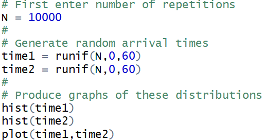
Here I will present code written in R*. I like to use N for the number of repetitions, which the user specifies before running the code. We can generate the random arrival times, with a vector of length N for each person, so we do not need to use a loop. We can also produce graphs of the individual and joint distributions using:
* I confess at the outset that I am a novice programmer.
Before running this code, I ask students: Predict what the graphs, both the histograms and the scatterplots, will look like. Here are some results with 10,000 repetitions:
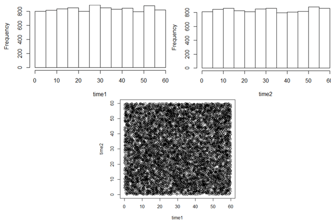
Describe what the histograms and scatterplots reveal. There’s not a lot to see here, but the histograms do confirm our expectations about uniform distributions. Also as expected, the scatterplot reveals random scatter throughout the 60×60 square of possible (joint) arrival times.
How can we calculate vectors of differences and absolute differences in arrival times? What do you expect histograms of these distributions to look like? The following code calculates these vectors and produces these graphs, and results are shown for 10,000 repetitions:
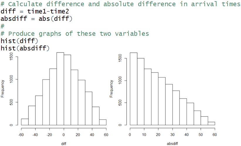
Describe what these graphs reveal. The distribution of differences in the graph on the left is quite symmetric about the value zero. This makes sense because the two people have the same distribution of arrival times. The graph on the right of the absolute differences results from folding the left side of the graph on the left about the zero axis. The distribution of absolute differences is certainly not symmetric. Smaller values for the absolute difference are more likely than larger values.
Now we’re ready to calculate an approximate probability to answer the question we started with. We just need to count how many of the repetitions produced an absolute difference in arrival times of 15 minutes or less. We can do this by creating a vector of true/false values, with TRUE meaning that they successfully met and FALSE meaning that they did not. We can do this with one line of code as follows, where the user needs to enter wait, the number of minutes that they agree to wait, before running the code:

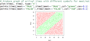
Next I like to re-produce the scatterplot above, making it more informative (and prettier!) by using different colors for whether the people successfully meet or not. Let’s use green for repetitions in which Eponine and Cosette successfully met and red for those in which they arrive so far apart that they do not meet. First I ask students: What do you expect the colored scatterplot to look like? In other words, where in the 60×60 square do you expect to see the green dots (where they successfully meet), and where do you expect to see the red dots (where they do not meet)? This question can be challenging, so I offer a hint: Where in the graph do they arrive at precisely the same time, in which case they certainly meet? Then I follow up with another hint: How far from that line can they arrive and still successfully meet? Here is some code and resulting graph for 10,000 repetitions:
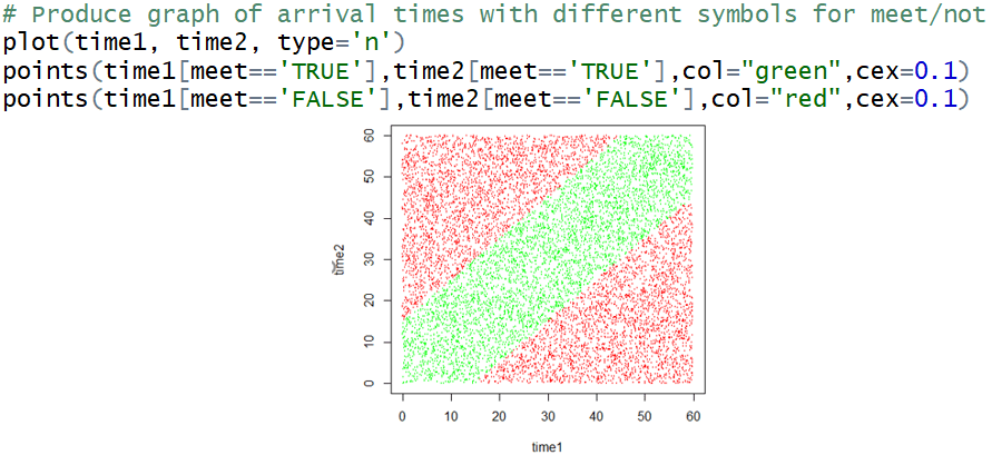
I think this is a beautiful graph*. It shows that Eponine and Cosette successfully meet if their joint arrival times are within 15 minutes above or below the y = x diagonal line. Next I ask: Based on this graph, make a guess for the probability that they successfully meet.
* I always tell my students that this graph would look great on a t-shirt, but so far none have taken the hint to produce such a t-shirt for me.
Now we are ready to calculate this probability (approximately) from the simulation results. We need to count how many repetitions result in a successful meeting. We can accomplish this by summing the vector of TRUE/FALSE values, because R treats TRUE as 1 and FALSE as 0. Then we divide by the number of repetitions to calculate the approximate probability. Here is the code and sample output for 10,000 repetitions:
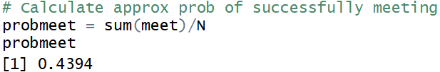
Calculate the margin-of-error associated with this approximate probability. Use the margin-of-error to determine a confidence interval for the actual long-run probability. In the beginning of a probability course, I give students the short-hand formula 1/sqrt(N) for the margin-of-error of an approximate probability based on a simulation analysis with N repetitions. With 10,000 repetitions, this produces a margin-of-error of .01, so we can be confident that the actual long-run probability is within the interval 0.4394 ± 0.0100, which is the interval (0.4294 à 0.4494). Eponine and Cosette have a slightly less than 50% chance of successfully meeting for lunch.
Eponine and Cosette might be disheartened to learn that they are more likely not to meet than to meet. Suppose that they want to change their waiting time to produce a 50% chance of meeting. Again I ask students to start with intuition: Do they need to increase or decrease their waiting time to achieve this 50% goal? Make a guess for how long they need to wait to have a 50% chance of successfully meeting.
Then I ask students: How can we use the simulation results to approximate how long they need to wait to produce a 50% chance of successfully meeting? This can be challenging, so I have hints ready: Which of the vectors that we generated is most relevant to this question? What aspect of that vector will approximate a 50% probability? Students eventually recognize that they can approximate the necessary waiting time with the median of the absolute differences in arrival times. Here’s the code and some sample output:
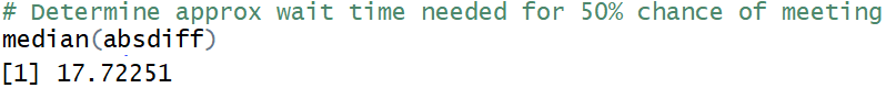
Because waiting 15 minutes produced a slightly smaller than 50% chance of a successful meeting, it makes sense that the approximate wait time for a 50% chance is a bit larger than 15 minutes.
Before we move on from simulation to a mathematical analysis, I return to a 15-minute wait time and ask: How can we improve the approximate probability? Students are quick to respond that using more repetitions should improve the approximation. Simulating one million repetitions produced an approximate probability of 0.437847. The margin-of-error is 1/sqrt(1,000,000) = 0.001, so a 95% confidence interval for the exact probability of a successful meeting is 0.437847 ± 0.001, which is the interval (0.436847 à 0.438847). The approximate wait time needed for a 50% chance of meeting turned out to be 17.60137 minutes.
With one million repetitions, the colored scatterplot of arrival times looks like:
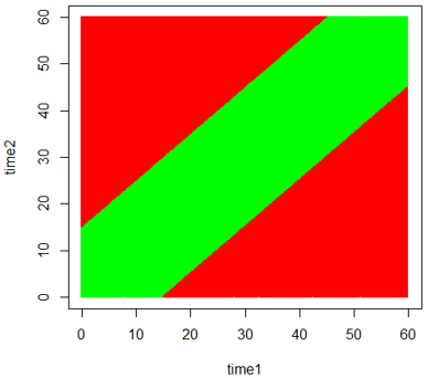
There are so many green and red dots in this graph that you cannot see the individual dots, but you can see a very clear image of the (green) region for which a successfully meeting occurs. This region provides the key to using geometry to calculate the exact probability.
Because the arrival distributions are independent and uniform, we can determine the exact probability of a successful meeting by calculating the area of the region in which they meet as a fraction of the total area of the region of possible (joint) arrival times. In other words, we need to calculate the probability that a point selected at random from the 60×60 square falls within the green region rather than one of the red regions.
Determine the area of the overall square. I often advise students that the denominator is typically easier to calculate with such probability questions. The area of the 60×60 square of possible (joint) arrival times is 60×60 = 3600 (in units of minutes squared).
Determine the area of the green region where they successfully meet. When students do not think of a shortcut from themselves, I offer a hint that makes this much easier: First determine the area of the red regions where they do not meet. The two red triangles have the same area, because both have a length of 45 minutes and height of 45 minutes. The area of each triangle is therefore 45×45/2 = 1012.5 (again in units of minutes squared), so the combined area of the two red triangles is 45×45 = 2025. The area of the green region is therefore 3600 – 2025 = 1575.
Use the areas to calculate the (exact, theoretical) probability that Eponine and Cosette successfully meet. This probability is 1575/3600 = 7/16 = 0.4375.
Are the two approximate probabilities from the simulation analyses above within the margin-of-error of the exact probability? Yes, the simulation with 10,000 repetitions produced an interval estimate of .4394 ± .0100, which is the interval (.4294 à .4494). The simulation with 1,000,000 repetitions produced an interval estimate of .437847 ± .001, which is the interval (.436847 à .438847). Both of these intervals include the exact probability of .4375.
Now let’s use geometry and algebra to determine how many minutes they must agree to wait, in order to have a 50% chance of successfully meeting. First I ask students: Express the probability of a successful meeting as a function of the number of minutes that each person agrees to wait. I suggest that students use Pr(S) to denote the probability of a successful meeting, and let m represent the number of minutes that each person agrees to wait. Again I have a hint ready: Start with a sketch of the 60×60 square. Then sketch the region where they meet, much like before, but using m rather than 15 as the number of minutes that they wait. Here’s a sketch:
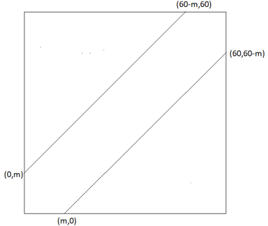
Each triangle now has length (60 – m) and height (60 – m), so its area is (60-m)×(60-m)/2. The combined area of the two triangles is therefore (60-m)×(60-m). The area of the non-triangular region where they successfully meet is then 3600 – (60-m)×(60-m). The probability of a successful meeting can be expressed as:
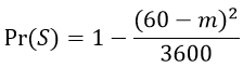
Graph this probability as a function of m, for values of m from 0 to 60 minutes. Some R code and output for this graph are:
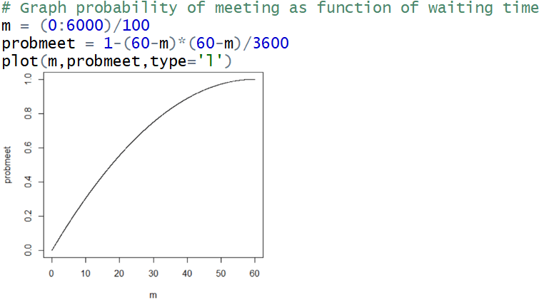
Describe the behavior of this function. Students should comment that this function is increasing, which certainly makes sense because waiting longer increases the probability of meeting. They should also observe that the rate of increase diminishes as the number of minutes increases. I also ask students to check that the probability for a 15-minute wait looks to be consistent with what we calculated earlier: .4375.
Now we are ready to do the algebra to solve for how long to wait in order to have a 50% chance of meeting. Setting Pr(S) = 0.5 produces (60-m)×(60-m) = 1800. Solving gives: m ≈ 17.5736 minutes. This value is very consistent with our approximate values from the simulation analyses above.
This activity can lead students to use intuition, simulation, and mathematics to solve probability problems. Unlike many probability problems that rely on combinatorics or calculus, geometry provides the solution to this one. Depending on your student audience and course goals, you could also ask students to do some coding themselves with this activity. You might also use this as an assignment rather than an in-class activity.
More extensions to this random rendezvous naturally present themselves. For example, we need not have assumed that Eponone’s and Cosette’s arrival times were uniformly distributed. How would the probability of a successful meeting change if their arrival times followed independent normal distributions? That depends on the means and standard deviations, which could be the same for both people or not. What if those normal distributions were not independent? We’ll consider those extensions in next week’s post, in which we will again use intuition, simulation, and mathematics to tackle probability questions.
P.S. This activity was inspired by problem #26, called The Hurried Duelers, in Frederick Mosteller’s wonderful book Fifty Challenging Problems in Probability.
P.P.S. The link below contains a file with the R code used above.


Trackbacks & Pingbacks