#22 Four more exam questions
In last week’s post (here), I presented twenty multiple choice questions, all conceptual in nature, none based on real data. This week I present four free-response questions that I have used on exams, all based on real data from genuine studies. These questions assess students’ abilities to draw and justify appropriate conclusions. Topics covered include confounding, biased sampling, simulation-based inference, statistical inference for comparing two groups, and cause-and-effect conclusions. All of these questions have multiple parts*. I also provide comments on the goal of each question and common student errors. I do not intend these four questions to comprise a complete exam. As always, questions for students appear in italics.
* I could have titled this post “Twenty more exam questions” if I had counted each part separately.
1. (6 pts) Researchers found that people who used candy cigarettes as children were more likely to become smokers as adults, compared to people who did not use candy cigarettes as children.
- (a) (1 pt) Identify the explanatory variable.
- (b) (1 pt) Identify the response variable.
- (c) (4 pts) When hearing about this study, a colleague of mine said: “But isn’t the smoking status of the person’s parents a confounding variable here?” Describe what it means for smoking status to be a confounding variable that provides an alternative to drawing a cause/effect explanation in this context.
Describing what confounding means can be very challenging for students. The key is to suggest a connection between the confounding variable and both the explanatory and response variables. I’ve tried to make this task as straight-forward as possible here. Students do not need to suggest a confounding variable themselves, and the context does not require specialized knowledge to explain the confounding.
Parts (a) and (b) are meant to be helpful by directing students to think about the explanatory and response variables in this study (and also offering an opportunity to earn two relatively easy points). The explanatory variable is whether or not the person used candy cigarettes as a child, and the response variable is whether or not the person became a smoker as an adult.
To earn full credit for part (c), students need to say something like:
- Parents who smoke are more likely to allow their children to use candy cigarettes than parents who do not smoke.
- Children of parents who smoke are more likely to become smokers as adults than children of parents who do not smoke.
It would be nice for students to add that these two connections would result in a higher proportion of smokers among those who used candy cigarettes as children than among those who did not use candy cigarettes, but I do not require such a statement.
Many students earn partial credit by giving only one of the two connections. Such a response fails to explain confounding fully and falls short of providing an alternative explanation for the observed association. Another common error is that some students focus on conjectured explanations, such as proposing only that children of smokers want to emulate their parents by using candy cigarettes, or that a genetic predisposition leads children of smokers to become smokers themselves. Both of these explanations come up short because they only address one of the two connections.
I sometimes make this question a bit easier by provide one of the connections for students: My colleague also pointed out that children of smokers are more likely to become smokers as adults than children of non-smokers. What else does the colleague need to say to complete the explanation of how parents’ smoking status is a confounding variable in this study? At other times I make this question harder by asking students to propose a potential confounding variable and also explain how the confounding could provide an alternative to a cause-and-effect explanation.
I sometimes make this question a bit easier by provide one of the connections for students: My colleague also pointed out that children of smokers are more likely to become smokers as adults than children of non-smokers. What else does the colleague need to say to complete the explanation of how parents’ smoking status is a confounding variable in this study? At other times I make this question harder by asking students to propose a potential confounding variable and also explain how the confounding could provide an alternative to a cause-and-effect explanation.
2. (8 pts) The news website CNN.com has posted poll questions that people who view the website can respond to. The following results were posted on January 10, 2012:
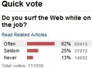
The margin-of-error, for 95% confidence, associated with this poll can be calculated to be ± .003, or ± 0.3%.
- a) (1 pt) Are the percentages reported here (62%, 25%, 13%) parameters or statistics? Explain briefly.
- b) (1 pt) Explain (using no more than ten words) why the margin-of-error is so small.
- c) (3 pts) Would you be very confident that between 61.7% and 62.3% of all employed Americans surf the Web often while on the job? Circle YES or NO. Also explain your answer.
Part (a) provides an easy point for students to earn by responding that these are statistics, because they are based on the sample of people who responded to the poll. Part (b) is also fairly easy; an ideal answer has only four words: very large sample size. I do not require that students report the sample size of 111,938. They can omit the word “very” and still earn full credit.
Part (c) is the key question. I want students to recognize that this poll relies on a very biased sampling method. Any online poll like this is prone to sampling bias, but the topic of this poll question especially invites bias. Only by surfing the web can a person see this poll question, so the sampling method favors those who surf the web often while at work. Because of this biased sampling method, students should not be the least bit confident that the population proportion is within the margin-of-error of the sample result.
I’ve learned to require students to circle YES or NO along with their explanation. Otherwise, several students try to have it both ways with a vague answer that tries to cover all possibilities, such as: I would be very confident of this, but I would also be cautious not to conclude anything too conclusively.
I used to present this poll result graphic to students and then ask specifically about sampling bias. But I changed to the above version, as I decided that it’s important for students to be able to spot sampling bias without being prompted to look for it.
3. (12 pts) Researchers presented young children with a choice between two toy characters who were offering stickers. One character was described as mean, and the other was described as nice. The mean character offered two stickers, and the nice character offered one sticker. Researchers wanted to investigate whether infants would tend to select the nice character over the mean character, despite receiving fewer stickers. They found that 16 of the 20 children in the study selected the nice character.
- a) (2 pts) Describe (in words) the null hypothesis in this study.
- b) (3 pts) Suppose that you were to conduct a simulation analysis of this study to investigate whether the observed result provides strong evidence that children genuinely prefer the nice character with one sticker over the mean one with two stickers. Indicate what you would enter for the following three inputs: i) Probability of success, ii) Sample size, iii) Number of samples.
- c) (1 pt) One of the following graphs was produced from a correct simulation analysis. The other two were produced from incorrect simulation analyses. Circle the correct one.
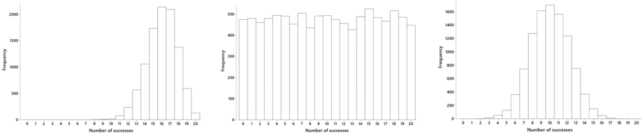
- d) (1 pt) Based on the correct graph, which of the following is closest to the p-value of this test: 5.000, 0.500, 0.050, 0.005? (Circle your answer.)
- e) (2 pts) Write an interpretation of the p-value in the context of this study.
- f) (3 pts) Summarize your conclusion from this research study and simulation analysis.
I am often asked about how to assess students’ knowledge of simulation-based inference* without using technology during the exam. This question shows one strategy for achieving this. Students need to specify the input values that they would use for the simulation, pick out what the simulation results would look like, estimate the p-value from the simulation results, and summarize an appropriate conclusion.
* See post #12 (here) for an introduction to simulation-based inference.
For part (a), I am looking for students to say that the null hypothesis is that children have no preference for either character. At this point I am not asking for students to express this hypothesis in terms of a parameter. It’s fine for them to state that children are equally likely to select either character, or that children select a character at random.
Correct responses for part (b) are to use 0.5 for the probability of success, 20 for the sample size, and a large number such as 1000 or 10,000 for the number of samples. Some students enter 0.8 for the probability of heads, based on the sample proportion of successes. A few students enter 20 for the number of repetitions.
Part (c) requires some thought, because my students have not seen such a question before. Some mistakenly think that the simulation results should be centered at the observed value, so they incorrectly select the graph on the left. The simulation results should be centered on what’s expected under the null hypothesis, as in graphs in the middle and on the right. Most students realize that they’ve never seen a simulation result look like the nearly-uniform distribution in the middle graph. Most recognize that they have frequently seen simulation results that look like the bell-shaped graph on the right, so they correctly select it.
To answer part (d) correctly, students need to be looking at the correct graph. For the graph on the right, very few of the repetitions produced 16 or more successes in 20 trials, so the p-value is very small. The smallest p-value among the options, .005, is the correct answer.
Many students struggle somewhat with part (e). One of the things that I like about the simulation-based approach to statistical inference is that I think it makes the interpretation of p-value as clear as possible. Students do not need to memorize an interpretation; they just need to describe what they see in the graph and remember the assumption behind the simulation analysis: If children had no preference between the characters, then only about 5 in 1000 (.005) repetitions would produce 16 or more successes. Many students get the second part of this interpretation correct but forget to mention the “if there were no preference” assumption; such a response earns partial credit. Sometimes I make this part of the question easier by giving a parenthetical hint: probability of what, assuming what?
Part (f), which is much more open-ended than previous parts, asks students to draw an appropriate conclusion. This study provides very strong evidence that children genuinely prefer the nice character over the mean character despite receiving fewer stickers from the nice character. This conclusion follows from the very small p-value, which establishes that it would be very surprising for 16 or more of 20 children to select the nice character, if in fact children had no preference for either character.
4. (16 pts) The Gallup organization released a report on October 20, 2014 that studied the daily lives and well-being of a random sample of American adults. The report compared survey responses between adults with children under age 18 living in the home and those without such children living in the home. The following table was provided in the report:
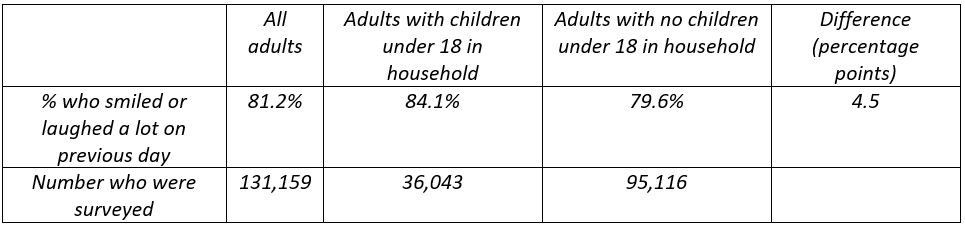
- a) (2 pts) Does this study involve random sampling, random assignment, both, or neither? Explain briefly.
- b) (2 pts) State the appropriate null and alternative hypotheses (using appropriate symbols) for testing whether the two populations of adults differ with regard to the proportion who smiled or laughed a lot on the previous day.
- c) (2 pts) The value of the test statistic turns out to be z = 18.5. Write a sentence interpreting the value of this z-test statistic. (This is not asking for a test decision or conclusion based on the z-test statistic.)
- d) (2 pts) Would you reject the null hypothesis at the .01 significance level? Explain how your answer follows from the value of the z-test statistic.
- e) (2 pts) A 99% confidence interval based on the sample data turns out to be (.039 à .051). Interpret what this interval says in this context.
- f) (2 pts) Is this confidence interval consistent with your test decision (from part d)? Explain how you know.
- g) (2 pts) Give a very brief explanation for why this confidence interval is very narrow.
- h) (2 pts) Suppose that someone reads about this study and says that having children in the household causes a very large increase in the likelihood of smiling or laughing a lot. Would you agree with this conclusion? Explain why or why not.
Presenting the sample statistics in the form of this table is a bit non-conventional. This is certainly not a 2×2 table of counts that students are accustomed to seeing. This can confuse some at first, but I think it’s worthwhile for students to see and grapple with information presented in multiple ways.
Part (a) revisits the theme of posts #19 and #20, titled Lincoln and Mandela (here and here), about the distinction between random sampling and random assignment. Students should note that the question states that the sample was selected randomly. But the Gallup organization certainly did not perform random assignment, because it would not be sensible or practical to randomly assign which people have children in their household and which do not.
To answer part (b) correctly, students need to realize that the test requires comparing proportions between two groups. The null hypothesis is that American adults with children in their household have the same proportion who smiled or laughed a lot on the previous day as those without children in their household. This null hypothesis can be expressed in symbols* as:
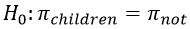
* Recall from post #13, titled A question of trust (here), that I like to use Greek letters for all parameter symbols, so I use π for a population proportion.
I could have asked students to calculate the z-test statistic, but part (c) provides this value and asks for an interpretation. I try to ward off a common error by cautioning students not to provide a test decision or conclusion. But many students do not know what interpreting the z-score means, even though we’ve done that often in class*. I want students to respond that the sample proportions (who smiled or laughed a lot on the previous day) in the two groups (those with/without children under age 18 in the household) are 18.5 standard deviations (or standard errors) apart. This is a huge difference. Students do not need to comment on the huge-ness until the next part, though. Despite my caution, many students draw a conclusion from the z-score here rather than interpret it. This could be because they do not read carefully enough, or it could well be that they do not understand what interpreting a z-score entails.
* See post #8, titled End of alphabet (here), for more thoughts and examples about z-scores.
For part (d), students should note that because the z-score of 18.5 is enormous, the p-value will be incredibly small, very close to zero. The tiny p-value leads to an emphatic rejection of the null hypothesis. Notice that I do not ask for an interpretation of this test decision in context here, only because parts (c) and (e) ask for interpretations.
Students need to realize that the confidence interval presented in part (e) estimates the difference in population proportions. I think this is fair to expect in part because that’s the conventional confidence interval to produce when comparing proportions between two groups, and also because the reported difference in sample proportions between the groups (.045) is the midpoint of the interval. We can be 95% confident that the proportion of American adults with a child under age 18 in the household is greater than the proportion among those without a child by between .039 and .051 (in other words by between 3.9 and 5.1 percentage points). Some students interpret this interval only as a difference without specifying direction (that those with a child are more likely to have smiled or laughed a lot). Such a response is only worth partial credit, because they’re leaving out an important element by not specifying which group has a higher proportion who smile or laugh a lot.
Part (f) is intended to be straightforward. Students should have rejected the null hypothesis that the population proportions are the same in the two groups. They should also notice that the confidence interval, containing only positive values, does not include zero as a plausible value for the difference in population proportions. These two procedures therefore give consistent results*.
* I hope that some students will remember the cat households example from post #16, titled Questions about cats (here), when they read this part. If they do, this recollection might also help with part (h) coming up.
Part (g) is asking about the very large sample size producing a narrow confidence interval. This is the same issue that I asked about in part (b) of question #2 about the CNN.com poll*.
* It’s certainly possible that I over-emphasize this point with my students.
I must admit that I really like part (h). The previous seven parts have been leading up to this part, which asks about the scope and type of conclusion students can draw from this survey. Notice that I use bold font for both causes and very large increase. This as a big hint that I want students to comment on both aspects. Most students correctly note that this is an observational study and not a randomized experiment, so a cause-and-effect conclusion (between having children in the household and being more likely to smile or laugh) is not justified. Relatively few students go on to address whether the difference between the groups is very large. I hope that they’ll look at the two sample proportions, and also at the confidence interval for the difference in population proportions, and then conclude that 3.9 to 5.1 percentage points does not indicate a very large difference between the two groups.
I hope these four exam questions, which aim to assess students’ abilities to draw and justify conclusions, provide a nice complement to last week’s multiple choice questions (here). See below for a link to a Word file containing these questions.
P.S. I thank my Cal Poly colleague Kevin Ross for introducing me to the Gallup poll and some good questions to ask about it. Kevin and his wife Amy have five children under age 18 in their household. I suspect that Kevin and his wife smile and laugh quite often.
P.P.S. The journal article on candy cigarette use can be found here. The article on children’s choices of toy characters can be found here; this is a follow-up study to a more well-known one that I often use in class, described here. A report on the Gallup survey about smiling and laughing can be found here.
P.P.P.S. Follow the link below for a Word file containing these four questions, and feel free to use or revise them for use with your own students.


Trackbacks & Pingbacks