#40 Back to normal

I presented some questions for helping students to understand concepts related to normal distributions in post #36 (here).  I return to normal distributions* in this post by presenting an extended activity (or assignment) that introduces the topic of classification and the concept of trade-offs in error probabilities.  This activity also gives students additional practice with calculating probabilities and percentiles from normal distributions.  As always, questions that I pose to students appear in italics.

* I came up with the “back to normal” title of this post many weeks ago, before so much of daily life was turned upside down by the coronavirus pandemic.  I realize that everyday life will not return to normal soon, but I decided to continue with the title and topic for this post.

---

Suppose that a bank uses an applicant’s score on some criteria to decide whether or not to approve a loan for the applicant.  Suppose for now that these scores follow normal distributions, both for people who would repay to the loan and for those who would not.  Those who would repay the loan have a mean of 70 and standard deviation of 8; those who not repay the loan have a mean of 30 and standard deviation of 8.

• a) Draw sketches of these two normal curves on the same axis. 
• b) Write a sentence or two comparing and contrasting these distributions.
• c) Suggest a decision rule, based on an applicant’s score, for deciding whether or not to give a loan to the applicant.
• d) Describe the two kinds of classification errors that could be made in this situation.
• e) Determine the probabilities of the two kinds of error with this rule.

a) Below is a graph, generated with R, of these two normal distributions.  The red curve on the left pertains to people who would not repay the loan; the green curve on the right is for those who would repay the loan:

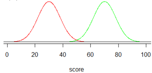
b) The two distributions have the same shape and variability.  But their centers differ considerably, with a much larger center for those who would repay the loan.  The scores show very little overlap between the two groups.

c) Most students have the reasonable thought to use the midpoint of the two means (namely, 50) as the cutoff value for a decision rule.  Some students need some help to understand how to express the decision rule: Approve the loan for those with a score of 50 or higher, and deny the loan to those with a score below 50.

d) This is the key question that sets up the entire activity.  Students need to recognize and remember that there are two distinct issues (variables) here: 1) whether or not the applicant would in fact repay the loan, and 2) whether the loan application is approved or denied.  Keeping these straight in one’s mind is crucial to understanding and completing this activity.  I find myself reminding students of this distinction often. 

With these two variables in mind, the two kinds of errors are:

• Denying the loan to an applicant who would repay
• Approving the loan for an applicant who would not repay

e) The z-scores are (50 – 70) / 8 = -2.50 for one kind of error and (50 – 30) / 8 = 2.50 for the other.  Both probabilities are approximately 0.006.  At this point I prefer that students use software* for these calculations, so they can focus on the concepts of classification and error probability trade-offs.  These probabilities are shown (but hard to see, because they are so small) in the shaded areas of the following graph, with cyan for the first kind of error and pink for the other:

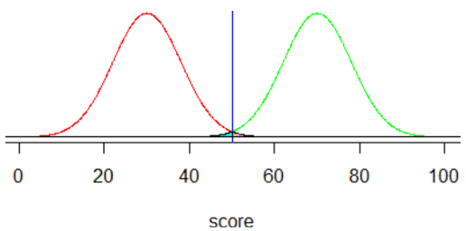
* Software options include applets (such as here), R, Minitab, Excel, …

---

More interesting questions arise when the two score distributions are not separated so clearly.

Now suppose that the credit scores are normally distributed with mean 60 and standard deviation 8 among those who would repay the loan, as compared to mean 40 and standard deviation 12 among those who would not repay the loan.

• f) Draw sketches of these two normal curves on the same axis.
• g) Describe how this scenario differs from the previous one.
• h) Determine the probabilities of the two kinds of error (using the decision rule based on a cut-off value of 50).
• i) Write a sentence or two to interpret the two error probabilities in context.

f) Here is the new graph:

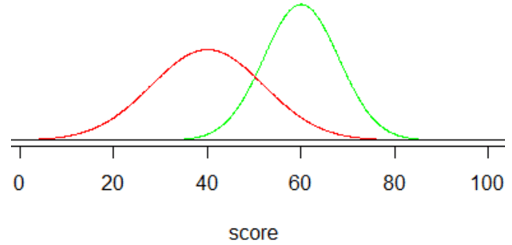
g) The primary change is that the centers of these score distributions are much closer than before, which means that the distributions have much more overlap than before.  This will make it harder to distinguish people who would repay their loan and those who would not.  A smaller difference is that the variability now differs in the two scores distributions, with slightly less variability in the scores of those who would repay the loan.

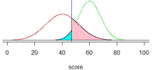
h) These error probabilities turn out to be approximately 0.106 for the probability that an applicant who would repay the loan is denied (shown in cyan in the graph below), 0.202 for the probability that an applicant who would not repay is approved (shown in pink):

i) I think this question is important for assessing whether students truly understand, and can successfully communicate, what they have calculated.  There’s a 10.6% chance that an applicant who would repay the loan is denied the loan.  There’s a 20.2% chance that an applicant who would not repay the loan is approved.

---

Now let’s change the cutoff value in order to decrease one of the error probabilities to a more acceptable level.

• j) In which direction – smaller or larger – would you need to change the decision rule’s cutoff value in order to decrease the probability that an applicant who would repay the loan is denied?
• k) How would the probability of the other kind of error – approving a loan for an applicant who would not repay it – change with this new cutoff value?
• l) Determine the cutoff value needed to decrease the error probability in (j) to .05.  Does this confirm your answer to (j)?
• m) Determine the other error probability with this new cut-off rule.  Does this confirm your answer to (k)?
• n) Write a sentence or two to interpret the two error probabilities in context.

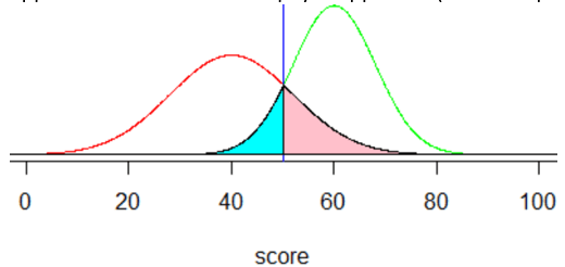
j) This question prompts students to think about the goal before doing the calculation.  This kind of error occurs when the score is less than the cutoff value, and we need the error probability to decrease from 0.106 to 0.050.  Therefore, we need a smaller cutoff value, less than the previous cutoff of 50.  Here is a graph of the situation, with the cyan-colored area reduced to 0.05:

k) Using a smaller cutoff value will produce a larger area above that value under the curve for people who would not repay the loan, as shown in pink in the graph above.  Therefore, the second error probability will increase as the first one decreases.

l) Students need to calculate a percentile here.  Specifically, they need to determine the 5^th percentile of a normal distribution with mean 60 and standard deviation 8.  They could use software to determine this, or they could realize that the z-score for the 5^th percentile is -1.645.  The new cutoff value needs to be 1.645 standard deviations below the mean: 60 – 1.645×8 = 46.84.  This is indeed smaller than the previous cutoff value of 50.  When students mistakenly add 1.645 standard deviations to the mean, I hope that they realize their error by recalling their correct intuition that the cutoff value should be smaller than before.

m) This probability turns out to be approximately 0.284, which is indeed larger than with the previous cutoff (0.202).

n) Now there’s a 5% chance that an applicant who would repay the loan is denied, because that’s how we determined the cutoff value for the decision rule.  This rule produces a 28.4% chance that an applicant who would not repay the loan is approved.

---

Now let’s reduce the probability of the other kind of error.

• o) Repeat parts (j) – (n) with the goal of decreasing the probability that an applicant who would not repay the loan is approved to 0.05.

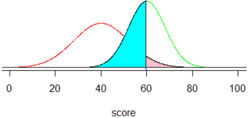
o) For this goal, the cutoff value needs to become larger than 50, which increases the probability that an applicant who would repay the loan is denied.  The cut-off value is now 1.645 standard deviations above the mean: 40 + 1.645×12 = 59.74.  This increases the other error probability to approximately 0.487.  This means that 48.7% of those who would repay the loan are denied, and 5% of those who would not repay are approved, as depicted in the following graph:

---

Now that we have come up with three different decision rules, I ask students to think about how we might compare them.

• p) If you consider the two kinds of errors to be equally serious, how might you decide which of the three decision rules considered thus far is the best?

This open-ended question is a tough one for students.  I give them a hint to think about the “equally serious” suggestion, and some suggest looking at the average (or sum) of the two error probabilities.

• q) Calculate the average of the two error probabilities for the three cutoff values that we have considered. 
• r) Which cutoff value is the best, according to this criterion, among these three options?

We can organize our previous calculations in a table:

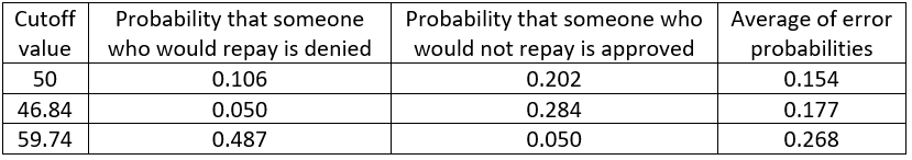
According to this criterion, the best cutoff value among these three options is 50, because that produces the smallest average error probability.  But of course, these three values are not the only possible choices for the cutoff criterion.  I suggest to students that we could write some code to calculate the two error probabilities, and their average, for a large number of possible cutoff values.  In some courses, I ask them to write this code for themselves; in other courses I provide them with the following R code:

• s) Explain what each line of code does.
• t) Run the code and describe the resulting graph.
• u) Report the optimal cutoff value and its error probabilities.
• v) Write a sentence describing the optimal decision rule.

Asking students to explain what code does is no substitute for asking them to write their own code, but it can assess some of their understanding:

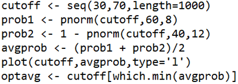
• The first line creates a vector of cutoff values from 30 to 70. 
• The second line calculates the probability that an applicant who would repay the loan has a score below the cutoff value and so would mistakenly be denied. 
• The third line calculates the probability that an applicant who would not repay the loan has a score above the cutoff value and so would mistakenly be approved. 
• The fourth line calculates the average of these two error probabilities. 
• The fifth line produces a graph of average error probability as a function of cutoff value. 
• The sixth line determines the optimal cutoff value by identifying which minimizes the average error probability. 

Here is the resulting graph:

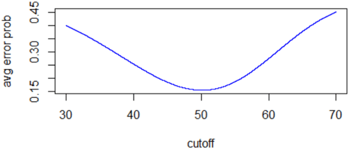
This graph shows that cutoff values in the neighborhood of 50 are much better (in terms of minimizing average error probability) than cutoff values less than 40 or greater than 60.  The minimum value of average error probability appears to be close to 0.15, achieved at a cutoff value slightly above 50.

The R output reveals that the optimal cutoff value is 50.14, very close to the first cutoff value that we analyzed.  With this cutoff value, the probability of denying an applicant who would repay the load is 0.109, and the probability of approving an applicant who would not repay is 0.199.  The average error probability with this cutoff value is 0.154. 

The optimal decision rule, for minimizing the average of the two error probabilities, is to approve a loan for those with a score of 50.14 or greater, and deny a loan to those with a score of less than 50.14.

• w) Now suppose that you consider denying an applicant who would repay the loan to be three time worse than approving an applicant who would not repay the loan.  What criterion might you minimize in this case?
• x) With this new criterion, would you expect the optimal cutoff value to be larger or smaller than before?  Explain.
• y) Describe how you would modify the code to minimize the appropriate weighted average of the error probabilities. 
• z) Run the modified code.  Report the optimal cutoff value and its error probabilities.  Also write a sentence describing the optimal decision rule.

We can take the relative importance of the two kinds of errors into account by choosing the cut-off value that minimizes a weighted average of the two error probabilities.  Because we consider the probability of denying an applicant who would repay to be the more serious error, we need to reduce that probability, which means using a smaller cutoff value.

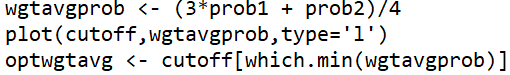
We do not need to change the first three lines of code.  The key change comes in the fourth line, where we must calculate a weighted average instead of an ordinary average.  Then we need to remember to use the weighted average vector in the fifth and sixth lines.  Here is the modified R code:

The graph produced by this code follows:

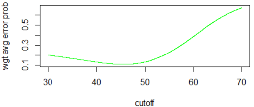
We see from the graph that the weighted average of error probabilities is minimized with a cutoff value near 45.  The R output reveals the optimal cutoff value to be 45.62.  The associated error probabilities are 0.036 for denying an applicant who would repay, 0.320 for approving an applicant who would not repay, and 0.107 for the weighted average.  The optimal decision rule for this situation is to approve applicants with a score of 45.62 or higher, deny applicants with a score of less than 45.62.

---

Whew, I have reached the end of the alphabet*, so I’d better stop there!

* You may have noticed that I had to squeeze a few questions into part (z) to keep from running out of letters.

Most teachers like to give their students an opportunity for lots of practice with normal distribution calculations.  With this activity, I have tried to show that you can provide such practice opportunities while also introducing students to ideas such as classification and error probability trade-offs. 

P.S. I have used a version of this activity for many years, but I modified the context for this blog post after watching a session at the RStudio conference held in San Francisco at the end of January.  Martin Wattenberg and Fernanda Viegas gave a very compelling presentation (a recording of which is available here) in which they described an interactive visualization tool (available here) that allows students to explore how different cutoff values affect error probabilities.  Their tool addresses issues of algorithmic fairness vs. bias by examining the impact of different criteria on two populations – labeled as blue and orange people.

P.P.S. I was also motivated to develop this activity into a blog post by a presentation that I saw from Chris Franklin in Atlanta in early February.  Chris presented some activities described in the revised GAISE report for PreK-12 (the updated 2020 version will appear here later this year), including one that introduces the topic of classification.