#48 My favorite problem, part 2

Now we continue with the analysis of my favorite problem, which I call “choosing the best,” also known as the “secretary problem.”  This problem entails hiring a job candidate according to a strict set of rules.  The most difficult rules are that you can only assess candidates’ quality after you have interviewed them, you must decide on the spot whether or not to hire someone and can never reconsider someone that you interviewed previously, and you must hire the very best candidate or else you have failed in your task.

Here’s a reminder of the outline for this three-part series:

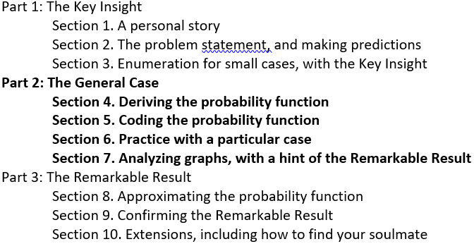
In the previous post (here), we analyzed some small cases by hand and achieved the Key Insight that led to the general form of the optimal solution: Let a certain number of candidates go by, and then hire the first candidate you see who is the best so far.  The question now is how many candidates to let pass before you begin to consider hiring one.  We’ll tackle the general case of that question in this post, and we’ll consider cases as large as 5000 candidates. 

I tell students that the derivation of the probability function in section 4 is the most mathematically challenging section of this presentation.  But even if they struggle to follow that section, they should be able to understand the analysis in sections 6 and 7.  This will provide a strong hint of the Remarkable Result that we’ll confirm in the next post.

Before we jump back in, let me ask you to make predictions for the probability of successfully choosing the best candidate, using the optimal strategy, for the numbers of candidates listed in the table (recall that the last number is the approximate population of the world):

As always, questions that I pose to students appear in italics.

---

4. Deriving the probability function

We need to figure out, for a given number of candidates, how many candidates you should let pass before you actually consider hiring one.  This is where the math will get a bit messy.  Let’s introduce some symbols to help keep things straight:

• Let n represent the number of candidates.
• Let i denote the position in line of the best candidate.
• Let r be the position of first “contender” that we actually consider hiring.
  • The strategy is to let the first (r – 1) candidates go by, before you genuinely consider hiring one.

We will express the probability of successfully choosing the best candidate as a function of both n and r.  After we have done that, then for any value of n, we can evaluate this probability for all possible values of r to determine the value that maximizes the probability.

First we will determine conditional probabilities for three different cases.  To see why breaking this problem into cases is helpful, let’s reconsider the n = 4 situation that we analyzed in the previous post (here).  We determined that the “let 1 go by” strategy is optimal, leading to success with 11 of the 24 possible orderings.  What value of r does this optimal strategy correspond to?  Letting 1 go by means that r = 2 maximizes the probability of success when n = 4.

These 24 orderings are shown below.  The ones that lead to successfully choosing the best with the “let 1 go by” strategy are displayed in green:

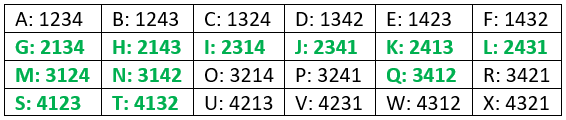
Looking more closely at our analysis of the 24 orderings with the “let 1 go by” (r = 2) strategy, we can identify different cases for how the position of the best candidate (i) compares to the value of r.  I’ve tried to use cute names (in italics below) to help with explaining what happens in each case:

• Case 1, Too soon (i < r): The best candidate appears first in line.  Because our strategy is to let the first candidate go by, we do not succeed for these orderings.  Which orderings are these?  A, B, C, D, E, and F.
• Case 2, Just right (i = r): The best candidate appears in the first position that we genuinely consider hiring, namely second in line.  We always succeed in choosing the best candidate in this circumstance.  Which orderings are these?  G, H, M, N, S, and T.
• Case 3a, Got fooled (i > r): The best candidate appears after the first spot at which we consider hiring someone.  But before we get to the best candidate, we get fooled into hiring someone else who is the best we’ve seen so far.  Which orderings are these?  O, P, R, U, V, W, and X.
• Case 3b, Patience pays off (also i > r): Again the best candidate appears after the first spot at which we consider hiring someone.  But now we do not get fooled by anyone else and so we succeed in choosing the best.  Which orderings are these?  I, J, K, L, and Q.

As we move now from the specific n = 4 case to the general case for any given value of n, we will consider the analogous three cases for how the position of the best candidate (i) compares to the value of r:

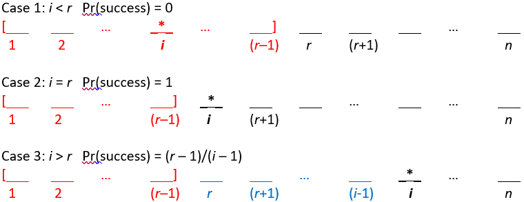
• Case 1: i < r, so the best candidate is among the first (r – 1) in line.  What is the probability that you successfully choose the best candidate in this case?  Remember that the strategy is to let the first (r – 1) go by, so the probability of success equals zero.  In other words, this is the unlucky situation in which the best candidate arrives while you are still screening candidates solely to gain information about quality.
• Case 2: i = r.  What is the probability that you successfully choose the best candidate in this case? When the best candidate is in position r, then that candidate will certainly be better than the previous ones you have seen, so the probability of success equals one.  This is the ideal situation, because the best candidate is the first one that you actually consider hiring.
• Case 3: i > r, so the best candidate arrives after you have started to consider hiring candidates*.  What is the probability that you successfully choose the best candidate in this case?  This is the most complicated of the three situations by far.  The outcome is not certain.  You might succeed in choosing the best, but you also might not.  Remember from our brute force analyses by enumeration that the problem is that you might get fooled into hiring someone who is the best you’ve seen but not the overall best.  What has to happen in order for you to get fooled like this?  In this situation, then you will succeed in choosing the best unless the best of the first (i – 1) candidates occurs after position (r – 1).  In this situation, you will be fooled into hiring that candidate rather than the overall best candidate.  In other words, you will succeed when the best among the first (i – 1) candidates occurs among the first (r – 1) that you let go by.  Because we’re assuming that all possible orderings are equally likely, the probability of success in this situation is therefore (r – 1) / (i – 1).

* This is the hardest piece for students to follow in the entire three-part post.  I always encourage them to take a deep breath here.  I also reassure them that they can follow along again after this piece, even if they do not understand this part completely.

The following diagrams may help student to think through these three cases.  The * symbol reveals the position of the best candidate.  The red region indicates candidates among the first (r – 1) who are not considered for hiring.  The blue region for case 3 contains candidates who could be hired even though they are not the very best candidate.

How do we combine these conditional probabilities to determine the overall probability of success?  When students need a hint, I remind them that candidates arrive in random order, so the best candidate is equally likely to be in any of the n positions.  This means that we simply need to take the average* of these conditional probabilities:

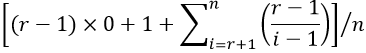
* This is equivalent to using the law of total probability.

This expression simplifies to:

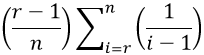
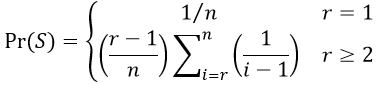
The above works for values of r ≥ 2.  The r = 1 situation means hiring the first candidate in line, so the probability of success is 1/n when r = 1.  Using S to denote the event that you successfully choose the best candidate, the probability function can therefore be written in general as:

Our task is now clear: For a given value of n, we evaluate this function for all possible values of r (from 1 to n).  Then we determine the value of r that maximizes this probability.  Simple, right?  The only problem is that those sums are going to be very tedious to calculate.  How can we calculate those sums, and determine the optimal value, efficiently?  Students realize that computers are very good (and fast) at calculating things over and over and keeping track of the results.  We just need to tell the computer what to do.

---

5. Coding the probability function

If your students have programming experience, you could ask them to write the code for this task themselves.  I often give students my code after I first ask some questions to get them thinking about what the code needs to do: How many loops do we need?  Do we need for loops or while loops?  What vectors do we need, and how long are the vectors? 

We need two for loops, an outer one that will work through values of r, and an inner one that will calculate the sum term in the probability function.  We also need a vector in which to store the success probabilities for the various values of r; that vector will have length n.

I also emphasize that this is a different use of computing than we use in much of the course.  Throughout my class, we make use of computers to perform simulations.  In other words, we use computers to generate random data according to a particular model or process.  But that’s not what we’re doing here.  Now we are simply using the computer to speed up a very long calculation, and then produce a graph of the results, and finally pick out the maximum value in a list.

Here is some R code* that accomplishes this task:

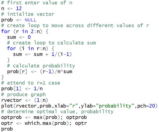
* A link to a file containing this code appears at the end of this post.

We figured out the n = 4 case by analyzing all 24 orderings in the last post (here), so let’s first test this code for that situation.  Here’s the resulting output:

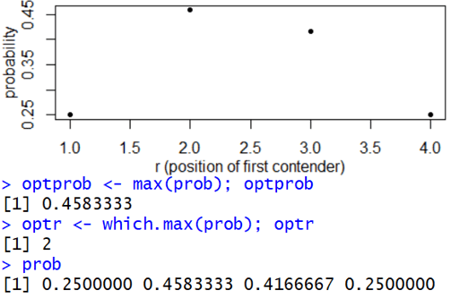
Explain how this graph is consistent with what we learned previously.  We compared the “let 1 go by” and “let 2 go by” strategies.  We determined the probabilities of successfully choosing the best to be 11/24 ≈ 0.4583 and 10/24 ≈ 0.4167, respectively.  The “let 1 go by” strategy corresponds to r = 2, and “let 2 go by” means r = 3.  Sure enough, the probabilities shown in the graph for r = 2 and r = 3 look to be consistent with these probabilities.  Why does it make sense that r = 1 and r = 4 give success probabilities of 0.25?  Setting r = 1 means always hiring the first candidate in line.  That person will be the best with probability 1/4.  Similarly, r = 4 means always hiring the last of the four candidates in line, so this also has a success probability of 1/4.

Let’s do one more test, this time with n = 5 candidates, which I mentioned near the end of the previous post.  Here’s the output:

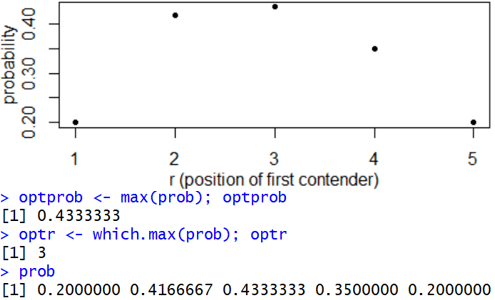
Based on this output, describe the optimal strategy with 5 candidates.  Is this consistent with what I mentioned previously?  Now the value that maximizes the success probability is r = 3.  The optimal strategy is to let the first two candidates go by*; then starting with the third candidate, hire the first one you encounter who is the best so far.  This output for the n = 5 case is consistent with what I mentioned near the end of the previous post.  The success probabilities are 24/120, 50/120, 52/120, 42/120, and 24/120 for r = 1, 2, 3, 4, and 5, respectively.

* Even though I keep using the phrase “go by,” this means that you assess their quality when you interview those candidates, because later you have to decide whether a candidate is the best you’ve seen so far.

---

6. Practice with a particular case

Now consider the case of n = 12 candidates, which produces this output:

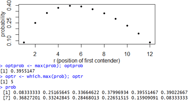
Describe the optimal strategy.  The value r = 5 maximizes the success probability when n = 12.  The optimal strategy is therefore to let the first 4 candidates go by and then hire the first one you find who is the best so far.  What percentage of the time will this strategy succeed in choosing the best?  The success probability with this strategy is 0.3955, so this strategy will succeed 39.55% of the time in the long run.  How does this probability compare to the n = 5 case?  This probability (of successfully choosing the best) continues to get smaller as the number of candidates increases.  But the probability has dropped by less than 4 percentage points (from 43.33% to 39.55%) as the number of candidates increased from 5 to 12.

To make sure that students understand how the optimal strategy works, I ask them to apply the strategy to the following 25 randomly generated orderings (from the population of 12! = 479,001,600 different orderings with 12 candidates).  This exercise can also be helpful for understanding the three cases that we analyzed in deriving the probability function above.  For each ordering, determine whether or not the optimal strategy succeeds in choosing the best candidate. 

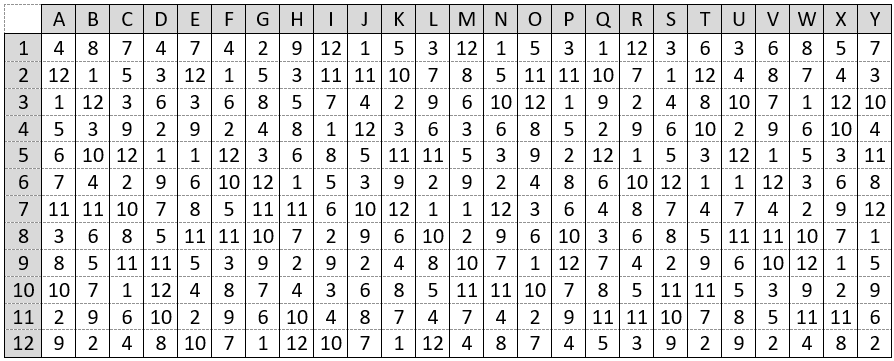
I typically give students 5-10 minutes or so to work on this, and I encourage them to work in groups.  Sometimes we work through several orderings together to make sure that they get off to a good start.  With ordering A, the best candidate appears in position 3, so our let-4-go-by strategy means that we’ll miss out on choosing the best.  The same is true for ordering B, for which the best candidate is in position 2.  With ordering C, we’re fooled into hiring the second-best candidate sitting in position 6, and we never get to the best candidate, who is back in position 10.  Orderings D and E are both ideal, because the best candidate is sitting in the prime spot of position 5, the very first candidate that we actually consider hiring.  Ordering F is another unlucky one in which the best candidate appears early, while we are still letting all candidates go by. 

I like to go slowly through ordering G with students.  Is ordering G a winner or a loser?  It’s a winner!  Why is it a winner when the best candidate is the very last one in line?  Because we got lucky with the second-best candidate showing up among the first four, which means that nobody other than the very best would be tempting enough to hire.

The following table shows the results of this exercise.  The numbers in bold color indicate which candidate would be hired.  Green letters and numbers reveal which orderings lead to successfully choosing the best.  Red letters and numbers indicate orderings that are not successful.

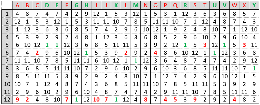
In what proportion of the 25 random orderings does the optimal strategy succeed in choosing the best candidate?  Is this close to the long-run probability for this strategy?  The optimal strategy resulted in success for 10 of these 25 orderings.  This proportion of 0.40 is very close to the long-run probability of 0.3955 for the n = 12 case from the R output.

---

7. Analyzing graphs, with a hint of the Remarkable Result

Now let’s run the code to analyze the probability function, and determine the optimal strategy, for larger numbers of candidates.  Here’s the output for n = 50 candidates:

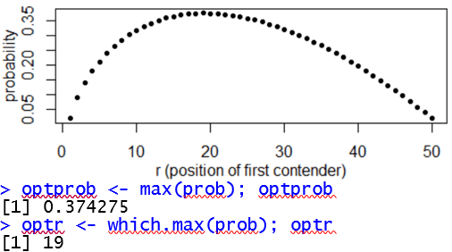
Describe the optimal strategy.  What is its probability of success?  How has this changed from having only 12 candidates?  The output reveals that the optimal value is r = 19, so the optimal strategy is to let the first 18 candidates go by and then hire the first one who is the best so far.  The probability of success is 0.3743, which is only about two percentage points smaller than when there were only 12 candidates.  How were your initial guesses for this probability?  Most students find that their initial guesses were considerably lower than the actual probability of success with the optimal strategy.

The graph on the left below shows how the optimal value of r changes as the number of candidates ranges from 1 to 50, and the graph on the right reveals how the optimal probability of success changes:

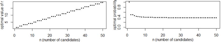
Describe what each graph reveals.  The optimal value of r increases roughly linearly with the number of candidates n.  This optimal value always stays the same for two or three values of n before increasing by one.  As we expected, the probability of success with the optimal strategy decreases as the number of candidates increases.  But this decrease is very gradual, much slower than most people expect.  Increasing the number of candidates from 12 to 50 only decreases the probability of success from 0.3955 to 0.3743, barely more than two percentage points.

---

Now consider output for the n = 500 (on the left) and n = 5000 (on the right) cases*:

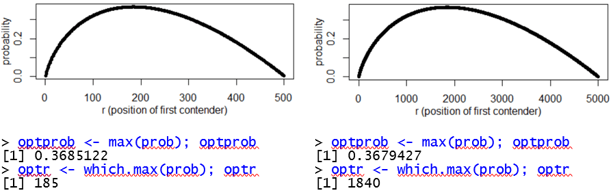
* The n = 5000 case takes only one second on my laptop.

What do these functions have in common?  All of these functions have a similar shape, concave-down and slightly asymmetric with a longer tail to the high end.   How do the optimal values of r compare?  The optimal values of r are 185 when n = 500 and 1840 when n = 5000.  By increasing the number of candidates tenfold, the optimal value of r increases almost tenfold.  In both cases, the optimal strategy is to let approximately 37% of the candidates go by, and then hire the first you see who is the best so far.  How quickly is the optimal probability of success decreasing?  This probability is decreasing very, very slowly.  Increasing the number of candidates from 50 to 500 to 5000 only results in the success probability (to three decimal places) falling from 0.374 to 0.369 to 0.368.

The following graphs display the optimal value of r, and the probability of success with the optimal strategy, as functions of the number of candidates:

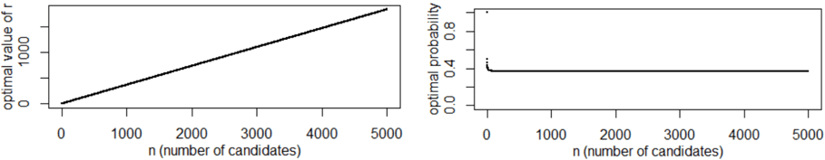
Describe what these graphs reveal.  As we noticed when we examined the graph up to 50 candidates, the optimal value of r continues to increase roughly linearly.  The probability of success with the optimal strategy continues to decrease at a very, very slow rate.

Some students focus so intently on answering my questions that they miss the forest for the trees, so I ask: Do you see anything remarkable here?  Yes!  What’s so remarkable?  The decrease in probability is so gradual that it’s hard to see with the naked eye in this graph.  Moreover, if 5000 candidates apply for your job, and your hiring process has to decide on the spot about each candidate that you interview, with no opportunity to ever go back and consider someone that you previously passed on, you can still achieve a 36.8% chance of choosing the very best candidate in the entire 5000-person applicant pool.

---

How were your guesses, both at the start of the previous post and the start of this one?

Let’s revisit the following table again, this time with probabilities filled in through 5000 candidates.  There’s only one guess left to make.  Even though the probability of choosing the best has decreased only slightly as we increase the number of candidates from 50 to 500 to 5000 candidates, there’s still a very long way to go from 5000 to almost 7.8 billion candidates!  Make your guess for the probability of successfully choosing the best if every person in the world applies for this job.

In the next post we will determine what happens as the number of candidates approaches infinity.  This problem provides a wonderful opportunity to apply some ideas and tools from single-variable calculus.  We will also discuss some other applications, including how you can amaze your friends and, much more importantly, find your soulmate in life!

---

P.S.  Here is a link to a file with the R code for evaluating the probability function: