#54 Probability without calculus or computation

This guest post has been contributed by Kevin Ross.  You can contact him at kjross@calpoly.edu.

Kevin Ross is a faculty colleague of mine in the Statistics Department at Cal Poly – San Luis Obispo.  Kevin is a probabilist who excels at teaching introductory statistics as well as courses in probability and theoretical statistics.  Kevin is a co-developer of a Python package called Symbulate (here) that uses the language of probability to conduct simulations involving probability models (described in a JSE article here).  I have borrowed examples and exam questions from Kevin on many occasions, so I am very glad that he agreed to write this guest post describing some of his ideas for assessing students’ knowledge of probability concepts without asking for calculations or derivations.

---

Allan still hasn’t officially defined what a “good question” is (see the very end of post #52, Top thirteen topics, here), but he’s certainly given many examples.  I’ll try to add to the collection by presenting four types of questions for assessing knowledge of probability:

1. Which is greater?
2. How would you simulate?
3. Sketch a plot
4. “Don’t do what Donny Don’t does”

I frequently use each type of question in class, on homework assignments, on quizzes, and on exams. I use questions like the ones throughout this post in introductory statistics courses and in upper division probability courses typically taken by majors in statistics, mathematics, engineering, and economics. One common theme is that the questions require no probability calculations.  I think these questions facilitate and assess understanding of probability concepts much better than questions that require calculus derivations or formulaic computations.

---

1. Which is greater?

This type of multiple choice question was first inspired by “Linda is a bank teller” and other studies of Daniel Kahneman and Amos Tversky that Allan mentioned in post #51 (Randomness is hard, here).  The following example illustrates the basic structure:

a) Which of the following – A or B – is greater? Or are they equal? Or is there not enough information to decide? (A) The probability that a randomly selected Californians likes to surf; (B) The probability that a randomly selected American is a Californian who likes to surf; (C) A and B are exactly the same; (D) Not enough information to determine which of A or B is greater

The structure is simple – two quantities A and B and the same four answer choices – but this framework can be used to assess a wide variety of concepts in probability. In all of the following examples, the prompt is: Which of the following – A or B – is greater? Or are they equal? Or is there not enough information to decide?

b) Randomly select a U.S. resident. Let R be the event that the person is a California resident, and let G be the event that the person is a Cal Poly graduate. (A) P(G|R); (B) P(R|G); (C) A and B are exactly the same; (D) Not enough information to determine which of A or B is greater

The answer to (a) is A because the sample space for A (Californians) is a subset of the sample space for B (Americans). The answer to (b) is B because although the two conditional probabilities have the same numerator, the denominator is smaller for the conditional probability in B than for the one in A.

I ask many versions of “what is the denominator?” questions like (a) and (b). Symbols can easily be interchanged with words. Also, “probability” can be replaced with “proportion” to assess proportional reasoning in introductory courses.

c) A fair coin is flipped 10 times. (A) The probability that the results are, in order, HHHHHHTTTT; (B) The probability that the results are, in order, HHTHTHHTT; (C) A and B are exactly the same; (D) Not enough information to determine which of A or B is greater

d) A fair coin is flipped 10 times. (A) The probability that the flips result in 6 Hs and 4 Ts; (B) The probability that the results are, in order, HHTHTHHTT; (C) A and B are exactly the same; (D) Not enough information to determine which of A or B is greater

Questions like (c) and (d) can assess the ability to differentiate between specific outcomes (six Hs followed by four Ts) and general events (six Hs in ten flips). Many students select B in (c) because the sequence “looks more random”, but the outcomes in A and B are equally likely. The answer to (d) is A because the sequence in B is only one of many outcomes that satisfy the event in A.

e) Shuffle a standard deck of 52 playing cards (of which 4 are aces) and deal 5 cards, without replacement. (A) The probability that the first card dealt is an ace; (B) The probability that the fifth card dealt is an ace; (C) A and B are exactly the same; (D) Not enough information to determine which of A or B is greater

Students find this question very tricky, but it gets at an important distinction between conditional versus unconditional probability (or independence versus “identically distributed”).  The correct answer is C, because in the absence of any information about the first 4 cards dealt, the unconditional probability that the fifth card is an ace is 4/52. (I like to use five cards rather than just two or three to discourage students from enumerating the results of the draws.)

f) A box contains 30 marbles, about half of which are green and the rest gold.  A sample of 5 marbles is selected at random with replacement.  X is the number of green marbles in the sample and Y is the number of gold marbles in the sample. (A) Cov(X, Y); (B) 0; (C) A and B are exactly the same; (D) Not enough information to determine which of A or B is greater

Many students select C, thinking that “with replacement” implies independence.  But while the individual draws are independent, the random variables X and Y have a negative correlation: If there is a large number of green marbles in the sample, then there must be necessarily a small number of gold ones.

g) E and F are events (defined on the same probability space) with P(E) = 0.7 and P(F) = 0.6. (A) 0.42; (B) P(E ꓵ F); (C) A and B are exactly the same; (D) Not enough information to determine which of A or B is greater

The answer would be C if the events E and F were independent. But that is not necessarily true, and without further information all we can say is that P(E ꓵ F) is between 0.3 and 0.6, so the correct answer is D.  I frequently remind students to be careful about assuming independence.

h) X, Y, and Z are random variables, each following a Normal(100, 10) distribution. (A) P(X + Y > 200); (B) P(X + Z > 200); (C) A and B are exactly the same; (D) Not enough information to determine which of A or B is greater

Some students select C, thinking that because Y and Z have the same distribution, then so do X + Y and X + Z.  However, X and Y do not necessarily have the same joint distribution as X and Z, and the joint distribution affects the distribution of the sum.  If X, Y, and Z were independent, then the answer would be C, but without that information (remember to be careful about assuming independence!) the answer is D.

i) X and Y are independent random variables, each following a Normal(100, 10) distribution. (A) X; (B) Y; (C) A and B are exactly the same; (D) Not enough information to determine which of A or B is greater

Some students select C, because X and Y have the same distribution.  But there are (infinitely) many potential values these random variables can take, so it’s impossible to know which one will be greater.  The following is a more difficult version of this idea; again, students often choose C but the correct answer is D.

j) X, Y, and Z are independent random variables, with X ~ Poisson(1), Y ~ Poisson(2), and Z~Poisson(3). (A) X + Y; (B) Z; (C) A and B are exactly the same; (D) Not enough information to determine which of A or B is greater

The last four examples illustrate two major themes behind many of the questions I ask in probability courses:

• Marginal distributions alone are not enough to determine joint distributions.
• Do not confuse a random variable with its distribution.

Many common mistakes in probability result from not heeding these two principles, so I think it’s important to give students lots of practice with these ideas and assess them frequently.

---

2. How would you simulate?

In virtually every probability problem I introduce, one of the first questions I ask is “how would you simulate?” Such questions are a great way to assess student understanding of probability distributions and their properties, and concepts like expected value or conditional probability, without doing any calculations.

a) Describe in detail how you could, in principle, perform by hand a simulation involving physical objects (coins, dice, spinners, cards, boxes, etc.) to estimate P(X = 5 | X > 2), where X has a Binomial distribution with parameters n=5 and p=2/7.  Be sure to describe (1) what one repetition of the simulation entails, and (2) how you would use the results of many repetitions.  Note: You do NOT need to compute any numerical values.

Here is a detailed response:

1. To simulate a single value of X, we can use the “story” for a Binomial distribution and think of X as counting the number of successes in 5 Bernoulli trials with probability of success 2/7.  To simulate a single trial, construct a spinner with 2/7 of the area shaded as success*.  To simulate a single value of X, spin the spinner 5 times and count the number of successes. If X > 2, record the value of X.  Otherwise, discard it and try again to complete step (1)**.
2. Repeat step (1) 10,000 times, to obtain 10000 values of X with X > 2.  Count the number of simulated values of X that are equal to 5 and divide by 10,000 to approximate P(X = 5 | X > 2).

* There are many possible randomization devices, including a seven-sided die or a deck of seven cards with two labeled as success.  However, it’s important that students implement independent trials, so they must indicate that cards are drawn with replacement.

** I also accept an answer that omits the “discard” part of step (1) and replaces step (2) with: Repeat step (1) 10,000 times to obtain 10,000 values of X.  Divide the number of simulated values of X that are equal to 5 by the number of simulated values of X that are greater than 2 to approximate P(X = 5 | X > 2).  Each method provides a point estimate of the conditional probability, but they differ with respect to simulation margin-of-error.  I discuss in class how the method which includes the “discard” part of step (1) is less computationally efficient but results in a smaller margin-of-error.

Students often write vague statements like “repeat this many times.”  But “this” could be a single spin of the spinner or a generating a single value of X. Therefore, it’s important that students’ responses clearly distinguish between (1) one repetition and (2) many repetitions. 

(b) Repeat (a) for the goal of estimating Cov(V, W), where V = X + Y, W = max(X, Y), and X, Y are i.i.d. Normal(100, 15). Assume that you have access to a Normal(0, 1) spinner.

Part (b) illustrates how tactile simulation can be used even with more advanced concepts like continuous or joint distributions.  I repeatedly use the analogy that every probability distribution can be represented by a spinner, like the following picture corresponding to a Normal(0, 1) distribution:

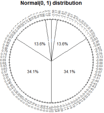
Notice how the values on the spinner are not evenly spaced; the sector corresponding to the range [0, 1] comprises 34.1% of the area while [1, 2] comprises 13.6%. (With more mathematically inclined students I discuss how to create such spinners by inverting cumulative distribution functions.) I have many clear plastic spinners that can be overlaid upon pictures like the above so students can simulate by hand values from a variety of distributions.

Here is a detailed response to part (b):

1. To simulate a single (V, W) pair: Spin the Normal(0, 1) spinner to obtain Z1, and let X = 100 + 15 × Z1. Spin the Normal(0, 1) spinner again to obtain Z2, and let Y = 100 + 15 × Z2. Add the X and Y values to obtain V = X + Y, and take the larger of X and Y to obtain W = max(X, Y). Record the values of V, W, and their product VW.
2. Repeat step (1) 10,000 times to obtain 10,000 values each of V, W, and VW.  Average the values of VW and subtract the product of the average of the V values and the average of the W values to approximate Cov(V, W).

I do think it’s important that students can write their own code to implement simulations.  But I generally prefer “describe in words” questions to “write the code” to avoid syntax issues, especially during timed exams.  When I want to assess student understanding of actual code on an exam, I provide the code and ask what the output would be. Of course, after discussing how to simulate and simulating a few repetitions by hand, we then carry out a computer simulation.  But before looking at the results, I often ask students to sketch a plot, as described in the next section.

---

3. Sketch a plot

As students progress in probability and statistics courses, they encounter many probability distributions but often have difficulty understanding just what all these distributions are.  Asking students to sketch plots, as in the following example, helps solidify understanding of random variables and distributions without any difficult calculus.

Suppose that X has a Normal(0, 1) distribution, U has a Uniform(-2, 2) distribution, X and U are independent, and Y = UX. For each of the following, sketch a plot representing the distribution.  The sketch does not have to be exact, but it should explicitly illustrate the most important features.  Be sure to clearly label any axes with appropriate values.  Explain the important features your plot illustrates and your reasoning*. (a) the conditional distribution of Y given U = -0.5; (b) the joint distribution of X and Y.

* I usually give full credit to well-drawn and carefully labeled plots regardless of the quality of explanation.  But “explaining in words” can help students who have trouble translating ideas into pictures.

Part (a) is not too hard once students realize they should draw a Normal(0, 0.5) density curve*, but it does take some thought to get to that point.  Even though the answer is just a normal curve, the question still assesses understanding of conditioning (treating U as constant) and the effect of a linear transformation.  The question also assesses the important difference between operations on random variables versus operations on distributions; it is X that is multiplied by -0.5, not its density. (Unfortunately, some students forget this and draw an upside-down normal curve.)

* However, I do deduct points if the variable axis isn’t labeled, or if the inflection points are not located at -0.5 and 0.5.  (The values on the density axis are irrelevant.)

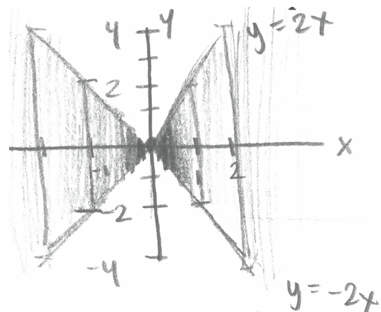
Part (b) is much harder. Here is an excellent student solution:

Students tend to find this type of question challenging, even after encountering examples in class activities and assignments. Here are some questions that I pose during class examples, which I hope students ask of themselves on assessments, to help them unpack these problems:

1. What is one possible plot point?  A few possible points? Students often have trouble even starting these problems, so just identifying a few possibilities can help.
2. What type of plot is appropriate? Since X and Y are two continuous random variables, a scatterplot or joint density plot is appropriate.
3. What are the possible values of the random variable(s)? After identifying a few possible values, I ask students to identify all the possible values and start labeling axes. Since X ~ Normal(0, 1), 99.7% of the values of X will fall between -3 and 3, so we can label the X-axis from -3 to 3.  (Remember, it doesn’t have to be perfect.) The value of Y depends on both X and U; identifying a few examples in step 1 helps students see how.  Given X = x, Y has a Uniform(-2|x|, 2|x|) distribution, so larger values of |x| correspond to more extreme values of Y.  Since most values of X lie between -3 and 3, most values of Y lie between -6 and 6, so we can label the Y-axis from -6 to 6.  But not all (X, Y) pairs are possible; only pairs within the region bounded by the lines y = 2x and y = -2x have nonzero density.  If students can make it to this point, drawing a plot with well-labeled axes and the “X-shaped” region of possible values, then they’ve made great progress.
4. What ranges of values are more likely?  Less likely? Values of X near 0 are more likely, and far from 0 are less likely.  Within each vertical strip corresponding to an x value, the Y values are distributed uniformly, so the density is stretched thinner over longer vertical strips. These observations help us shade the plot as in the example.

Determining an expression for the joint density in part (b) is a difficult calculus problem involving Jacobians.  Even students who are able to do the calculus to obtain the correct density might not be able to interpret what it means for two random variables to have this joint density.  Furthermore, even if students are provided the joint density function, they might not be able to sketch a plot or understand what it means. But I’m pretty confident that students who draw plots like the above have a solid understanding of concepts including normal distributions, uniform distributions, joint distributions, and transformations.

---

4. “Don’t do what Donny Don’t does”

This title is an old Simpson’s reference (see here). In these questions, Donny Don’t represents a student who makes many common mistakes. Students can learn from the common mistakes that Donny makes by identifying what is wrong and why, and also by helping Donny understand and correct his mistakes.

At various points in his homework, Donny Don’t writes the following expressions. Using simple examples, explain to Donny which of his statements are nonsense, and why. (A represents an event, X a random variable, P a probability measure, and E an expected value.) a) P(A = 0.5); b) P(A)∪ P(B); c) P(X); d) P(X = E(X)).

I’ll respond to Donny using tomorrow’s weather as an example, with A representing the event that it rains tomorrow, X tomorrow’s high temperature (in degrees F), and B the event that tomorrow’s high temperature is above 80 degrees.

(a) It doesn’t make sense to say “it rains tomorrow equals 0.5.” If Donny wants to say “the probability that it rains tomorrow equals 0.5” he should write P(A) = 0.5. (Mathematically, A is a set and 0.5 is a number, so it doesn’t make sense to equate them.)

(b) What Donny has written reads as “the probability that it rains tomorrow or the probability that tomorrow’s high temperature is above 80 degrees F,” which doesn’t make much sense.  Donny probably means “the probability that (it rains tomorrow) or (tomorrow’s high temperature is above 80 degrees),” which he should write as P(A ∪ B). (Mathematically, P(A) and P(B) are numbers while union is an operation on sets, so it doesn’t make mathematical sense to take a union of numbers.) Donny might have meant to write P(A) + P(B), which is valid expression since P(A) and P(B) are numbers. However, he should keep in mind that P(A) + P(B) is not necessarily a probability of anything; this sum could even be greater than one.  In particular, since there are some rainy days with high temperatures above 80 degrees, P(A) + P(B) is greater than P(A ∪ B).

(c) Donny has written “the probability that tomorrow’s high temperature,” which is a subject in need of a predicate.  We assign probabilities to things that could happen (events) like “tomorrow’s high temperature is above 80 degrees,” which has probability P(X > 80).

(d) Donny’s notation is actually correct!  Students often find this expression strange at first, but since E(X) represents a single number, P(X = E(X)) makes just as much sense as P(X = 80). Even if we don’t know the value of E(X), it still makes sense to consider “the probability that tomorrow’s high temperature is equal to the average high temperature.” Some students might object that X is continuous and so P(X = E(X)) = 0, but P(X = E(X)) is still a valid expression even when it equals 0.

Questions like this do more than encourage and assess proper use of notation.  Explaining to Donny why he is wrong helps students better understand the probabilistic objects that symbols represent and how they connect to real-world contexts.

---

I hope these examples demonstrate that even in advanced courses in probability or theoretical statistics, instructors can ask a variety of probability questions that don’t require any computation or calculus.  Such questions can not only assess students’ understanding of probability concepts but also help them to develop their understanding in the first place.  I have many more examples that I’d be happy share, so please feel free to contact me (kjross@calpoly.edu)!

P.S. Many thanks to Allan for having me as a guest, and thanks to you for reading!

This guest post has been contributed by Kevin Ross.  You can contact him at kjross@calpoly.edu.