#53 Random champions

This guest post has been contributed by Josh Tabor. You can contact him at TaborStats@gmail.com.

Josh Tabor teaches AP Statistics at Canyon del Oro High School in Oro Valley, Arizona, near Tucson*.  He is a co-author of a widely used textbook for AP Statistics, titled The Practice of Statistics.  He also co-wrote Statistical Reasoning in Sports, a textbook that uses simulation-based inference from the very first chapter.  Josh and I have worked together for many years at the AP Statistics Reading, and we have also presented at some of the same workshops and conferences.  Even more fun, we have attended some pre-season baseball games together in Arizona.  Josh is a terrific presenter and expositor of statistical ideas, so I am delighted that he agreed to bat lead-off for this series of guest bloggers.  Sticking with the baseball theme, he has written a post about randomness, simulation, World Series champions, teaching statistical inference, and asking good questions.

* Doesn’t it seem like the letters c and s are batting out of order in Tucson?

---

I am a big believer in the value of simulation-based inference, particularly for introducing the logic of significance testing. I start my AP Statistics class with a simulation-based inference activity, and try to incorporate several more before introducing traditional inference. Many of these activities foreshadow specific inference procedures like a two-sample z-test for a difference in proportions, but that isn’t my primary goal. Instead, my goal is to highlight how all significance tests follow the same logic, regardless of the type of data being collected. The example that follows doesn’t align with any of the tests in a typical introductory statistics class, but it is a fun context and helps achieve my goal of developing conceptual understanding of significance testing.

---

In a 2014 article in Sports Illustrated (here), author Michael Rosenberg addresses “America’s Wait Problem.” That is, he discusses how fans of some teams have to wait many, many years for their team to win a championship. In Major League Baseball, which has 30 teams, fans should expect to wait an average of 30 years for a championship—assuming all 30 teams are equally likely to win a championship each season. But is it reasonable to believe that all teams are equally likely to win a championship?

Rosenberg doesn’t think so. As evidence, he points out that in the previous 18 seasons, only 10 different teams won the World Series. Does having only 10 different champions in 18 seasons provide convincing evidence that the 30 teams are not equally likely to win a championship?

Before addressing whether the evidence is convincing, I start my students off with a (perhaps) simpler question:

• Rosenberg suggests that having 10 different champions in 18 seasons is evidence that teams are not equally likely to win a championship. How does this evidence support Rosenberg’s claim?

This isn’t the first time I have asked such a question to my students. From the beginning of the year, we have done a variety of informal significance tests, like the ones Allan describes in posts #12, #27, and #45 (here, here, and here). In most previous cases, it has been easy for students to identify how the given evidence supports a claim. For example, if we are testing the claim that a population proportion p > 0.50 and obtain a sample proportion of p-hat = 0.63, then recognizing that p-hat = 0.63 > 0.50 is very straightforward.

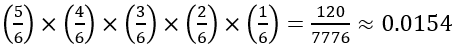
In this case, the statistic presented as evidence is quite different from a simple proportion or mean or even a correlation coefficient. Here the statistic is the number of different champions in an 18-year period of time. Some students will naively suggest that if teams are equally likely to win a championship, there should be 18 different champions in 18 seasons. And because 10 < 18, these data provide the evidence we are looking for. If students go down this path, you might ask a follow-up question: If you were to roll a die 6 times, would you expect to get 6 different results? If you have the time, you might even pull out a die and give it 6 rolls. (If you are nervous, there is less than a 2% chance of getting 6 different outcomes in 6 rolls of a fair die*.)

* This calculation is:

Once students are convinced that 18 is the wrong number to compare to, I pose a new question:

• If all 30 teams are equally likely to win a championship, what is the expected value of the number of different champions in 18 seasons?

There is no formula that I know of that addresses this question. Which leads to another question:

• What numbers of different champions (in 18 seasons) are likely to happen by chance alone, assuming all 30 teams are equally likely to win a championship?

Upon hearing the words “by chance alone,” my students know how to determine an answer: Simulation! Now for more questions:

• How can you simulate the selection of a World Series champion, assuming all teams are equally likely to win the championship?
• How do you conduct 1 repetition of your simulation?
• What do you record after each repetition of your simulation?

If we have time, I like students to work in groups and discuss their ideas. There are a variety of different approaches that students take to answer the first question: rolling a 30-sided die, with each side representing a different team; putting the names of the 30 teams in a hat, mixing them up, and choosing a team; or spinning 30-section spinner, with each section having the same area and representing one of the teams. I am happy when students think of physical ways to do the simulation, as that is what I have modeled since the beginning of the year. But I am also happy when they figure out a way to use technology: Generate a random integer from 1–30, where each integer represents a different team.

Assuming that students settle on the random integer approach, they still need to figure out how to complete one repetition of the simulation. In this case, they would need to generate 18* integers from 1–30, one integer (champion) for each season, allowing for repeated integers**. To complete the repetition, they must determine the value of the simulated statistic by recording the number of different integers in the set of 18. For example, there are 14 different champions in the following set of 18 random integers (repeat champions underlined): 22, 24, 17, 14, 8, 1, 11, 9, 25, 17, 17, 24, 16, 7, 18, 16, 30, 19.

* As I was brainstorming for this post, I started by counting the number of champions in the previous 30 MLB seasons, rather than the 18 seasons mentioned in the article. I didn’t want to be guilty of cherry-picking a boundary to help make my case. And 30 seemed like a nice number because it would allow for the (very unlikely) possibility of each team winning the championship once (not because of the central limit theorem!). But, using the same number in two different ways (30 teams, 30 seasons) is sure to create confusion for students. So I stuck with the 18-season window from the article.  Also, I realized that an 18-season window captures an entire lifetime for my students.

** Early in my teaching career (2001 to be precise), there was a simulation question on the AP Statistics exam that required students to account for sampling without replacement. Until then, we had always done examples where this wasn’t an issue. After 2001, I made a big deal about “ignoring repeats” until I realized that students were now including this phrase all the time, even when it wasn’t appropriate. I now try include a variety of examples, with only some requiring students to “ignore repeats.”  In this context of sports champions, of course, repeats are at the very heart of the issue we’re studying.

---

Once students have had the opportunity to share their ideas, we turn to technology to run the simulation. My software of choice for simulation is Fathom (here), but there are many alternatives. Here are the results of 10,000 repetitions of the simulation. That is, the results of 10,000 simulated sets of 18 seasons, assuming all 30 teams are equally likely to win the championship each year:

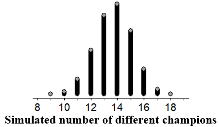
In this simulation of 10,000 seasons, the mean number of different champions is 13.71, and the standard deviation is 1.39. The minimum value is 9, and the maximum is 18, which indicates that every season had a different champion for at least one of the 10,000 simulated seasons.

Back to the questions:

• There is a dot at 9. What does this dot represent?

This is one of my very favorite questions to ask anytime we do a simulation. In this case, the dot at 9 represents one simulated 18-year period where there were 9 different champions.

• Using the results of the simulation, explain how having 10 champions in 18 seasons is evidence for Rosenberg’s claim that teams are not equally likely to win a championship.

Note that I am not asking whether the evidence is convincing. Yet. For now, I want students to notice that the expected number of different champions is 13 or 14 (expected value  13.71) when each team is equally likely to win the championship over an 18-year period. And most importantly, 10 is less than 13 or 14. So, Rosenberg’s intuition was correct when he cited the value of this statistic as evidence for his claim. Now that we have identified the evidence, I ask the following:

• What are some explanations for the evidence? In other words, what are some plausible explanations for why we got a value less than 14?

My students have already been through this routine several times, so they are pretty good about answering this question. And if they can provide the explanations in my preferred order*, I am especially happy.

• Explanation #1: All teams are equally likely to win the championship each year, and the results in our study happened by chance alone. Note that both clauses of this sentence are very important. My students always get the second half (“it happened by chance!”), but they also need the first part to have a complete explanation.
• Explanation #2: Teams aren’t equally likely to win the championship. In other words, some teams are more likely to win championships than others (sorry, Seattle Mariners fans!).

* This is my preferred order because it parallels the null and alternative hypotheses that we will discuss later in the year.

Once these two explanations are identified, we return to the original question:

• Does having 10 different champions in 18 seasons provide convincing evidence that all teams are not equally likely to win a championship?

For evidence to be convincing, we must be able to essentially rule out Explanation #1. Can we? To rule out Explanation #1, we need to know how likely it is to get evidence as strong or stronger than the evidence we found in our study, assuming that all teams are equally likely to win the championship each year.

• How can you use the dotplot to determine if the evidence is convincing?

When I am leading students through this discussion, there are usually a few who correctly respond “See how often we got a result of 10 or fewer by chance alone.” But when I ask similar questions on exams, many students don’t provide the correct answer. Instead, they give some version of the following: “Because nearly half of the dots are less than the mean, it is possible that this happened by chance alone.”* The use of the word “this” in the previous sentence points to the problem: students aren’t clear about what event they are supposed to consider. Once I started asking students to state the evidence at the beginning of an example, this error has occurred less often.  

* This is even more common when there is a clearly stated null hypothesis like H₀: p₁ – p₂ = 0 and students are tempted to say “because about half of the dots are positive…”

• In the simulation, 98 of the 10,000 simulated seasons resulted in 10 or fewer different champions, as highlighted in the graph below.  Based on this result, what conclusion would you make?

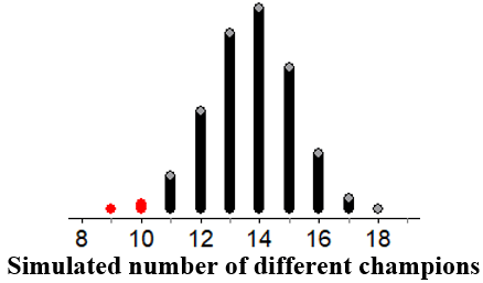
In the simulation, getting a result of 10 or fewer different champions was pretty rare, occurring only 98 times in 10,000 repetitions* (probability  0.0098). Because it is unlikely to get 10 or fewer different champions by chance alone when all 30 teams are equally likely to win the championship, there is convincing evidence that teams in this 18-year period were not equally likely to win the championship.

* Of course, this describes a p-value. I don’t call it a p-value until later in the year, but I am careful to use correct language, including the assumption that the null hypothesis is true.

---

As always, the scope of inference is important to consider. I also like to give students experience with raw data that allows them to determine the value of the statistic for themselves.  I remind students that the conclusion above was about “this 18-year period.” That is, the 18-year period prior to the article’s publication in November 2014. Here are the World Series champions for the 18-year period from 2002–2019*:

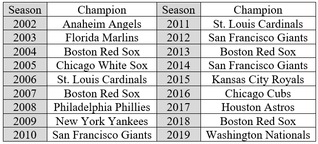
* In addition to matching the 18-year period length from the article, this allows me to include my favorite team in the list of World Series champions: Go Angels! It also makes me feel old as most of my current students weren’t even alive in 2002!

• What are the observational units for these sample data?  What is the variable?  What statistic will we determine from this sample?  What is the value of that statistic for this sample?

The observational units are the 18 seasons, and the variable is the World Series champion for that season. The statistic is the number of different champions in these 18 seasons. There were 12 different champions in this 18-year period. The repeat champions were the Boston Red Sox (4 times), San Francisco Giants (3 times), and St. Louis Cardinals (twice).

• To determine if these data provide convincing evidence that all teams are not equally likely to win a championship in 2002–2019, do we need to conduct a different simulation?

No. Because the number of seasons (18) and the number of teams (30) are still the same, we can use the results of the previous simulation to answer the question about 2002–2019.

• For the 18-year period from 2002–2019, is there convincing evidence that all teams are not equally likely to win a championship?

No. The graph of simulation results shows that a result of 12 or fewer different champions in 18 seasons is not unusual (probability  0.1916). Because it is not unlikely to get 12 or fewer different champions by chance alone, when all 30 teams are equally likely to win the championship each season, the data do not provide convincing evidence that teams in this 18-year period were not equally likely to win the championship. In other words, it is plausible that all 30 teams were equally likely to win the championship in the period from 2002–2019*.

* To avoid the awkward double negative in their conclusions, it is very tempting for students to include statements like the final sentence in the preceding paragraph. Unfortunately, they usually leave out wiggle phrases like “it is plausible that” or “it is believable that.” Once your students have had some experience making conclusions, it is important to caution them to never “accept the null hypothesis” by suggesting that there is convincing evidence for the null hypothesis.  In this context, no sports fan really believes that all teams are equally likely to win the championship each season, but the small sample size does not provide convincing evidence to reject that claim.

---

If you have the time and students seem interested in this topic, you can expand into other sports. Here are some questions you might ask about the National Football League:

• Do you think there would be stronger or weaker evidence that NFL teams from the previous 18 seasons aren’t equally likely to win a championship?

Most people expect the evidence to be stronger for the NFL. Even though the NFL tries to encourage parity, the New England Patriots seem to hog lots of Super Bowl titles.

• If we were to simulate the number of different champions in an 18-year period for the NFL, assuming all 32 teams are equally likely to win a championship, how would conducting the simulation differ from the earlier baseball simulation?

Instead of generating 18 integers from 1–30, we would generate 18 integers from 1–32.

• How do you think the results of the simulation would differ?

With more teams available to win the championship, the expected value of the number of different champions should increase.

• It just so happens that 12 different NFL teams have won a championship in the previous 18 seasons, the same as the number of MLB teams that have won a championship in the previous 18 seasons. (The Patriots won 5 of these championships.) Based on your answer to the previous question, would the probability of getting 12 or fewer NFL champions by chance alone be larger, smaller, or about the same as the probability in the MLB simulation (0.1916)?

This probability will be smaller, as the expected number of different champions in the NFL is greater than in MLB, so values of 12 or fewer will be less likely in the NFL simulation.

Here are the results of 10,000 simulated 18-season periods for the NFL:

The most common outcome is still 14 different champions, but the mean number of different champions increases from about 13.71 with MLB to about 13.94 with NFL. (The standard deviation also increases from 1.39 to 1.41).

The p-value for the NFL data is about 0.1495, smaller (as expected) than the p-value of 0.1916 for the MLB data. However, because the  p-value is not small, these data do not provide convincing evidence that the 32 NFL teams are not equally likely to win the championship each season.

---

Each time we do an informal significance test like this one, I rehearse the logic with my students:

1. Identify the statistic to be used as evidence, and explain why it counts as evidence for the claim being tested.
2. Describe the two explanations for the evidence.
3. Use simulation to explore what is likely to happen by chance alone.
4. Compare the evidence to what is likely to happen by chance alone. If it is unlikely to get evidence as strong as or stronger than the observed evidence, then the evidence is convincing.

P.S. Thanks to Allan for letting me share some thoughts in this post. And thanks for each of the 52 entries that precede this one!

This guest post has been contributed by Josh Tabor. You can contact him at TaborStats@gmail.com.