#70 Batch testing, part 2

I recently asked my students to analyze expected values with batch testing for a disease, which I discussed in some detail in post #39, here.  Rethinking this scenario led me to ask some new questions that I had not asked in that earlier post.

I will first re-introduce this situation, present the basic questions and analysis that my students worked through, and then ask the key question that I wish I had asked previously.  If you’d like to skip directly to the new part, scroll down to the next occurrence of “key question.” As always, questions that I pose to students appear in italics.

---

Suppose that 12 people need to be given a blood test for a certain disease.  Assume that each person has a 10% chance of having the disease, independently from person to person.  Consider two different plans for conducting the tests:

• Plan A: Give an individual blood test to each person.
• Plan B: Combine blood samples from all 12 people into one batch; test that batch.
  • If at least one person has the disease, then the batch test result will be positive, and then all 12 people will need to be tested individually.
  • If nobody has the disease, then the batch test result will be negative, and no additional tests will be needed.

Let the random variable X represent the total number of tests needed with plan B (batch testing).

a) Determine the probability distribution of X. [Hint: List the possible values of X and their probabilities.]

Even with the hint, some of my students were confused about where to begin, so I tried to guide them through the implications of the two sub-bullets describing how batch testing works.

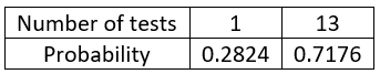
The possible values of X are 1 (if nobody has the disease) and 13 (if at least one person has the disease).  The probabilities are: Pr(X = 1) = Pr(nobody has the disease) = (.9)¹² ≈ 0.2824 by the multiplication rule for independent events, and Pr(X = 13) = 1 – Pr(nobody has the disease) = 1 – (.9)¹² ≈ 0.7176.  This probability distribution can be represented in the following table:

b) If you implement plan B once, what is the probability that the number of tests needed will be smaller than it would be with plan A?

This question really stumps some students.  Because plan A always requires 12 tests, the answer is simply: Pr(X < 12) ≈ 0.2824.  My goal is for students to realize that batch testing reduces the required number of tests only about one-fourth of the time, so this criterion does not reveal any advantage of batch testing.  Maybe I need to ask the question differently, or ask a different question altogether, to direct students’ attention to this point.

c) Determine the expected value of X.

This calculation is straightforward: E(X) = 1(.9)¹² + 13(1 – .9¹²) ≈ 9.61.

d) Interpret what this expected value means in this context.

My students quickly realize that I want them to focus on long-run average when they interpret expected value (see post #18, here).  But a challenging aspect of this is to describe what would be repeated a large number of times.  In this case: If the batch testing plan were applied for a very large number of groups of 12 people, then the long-run average number of tests needed would be very close to 9.61 tests.

e) Which plan – A or B – requires fewer tests, on average, in the long run?

Maybe I should have asked this differently, perhaps in terms of choosing between plan A and plan B.  The answer is that plan B is better in the long run, because it will require about 9.61 tests on average, compared to 12 tests with plan A.

---

Now consider a third plan:

• Plan C: Randomly divide the 12 people into two groups of 6 people each.  Within each group, combine blood samples from the 6 people into one batch.  Test both batches.
  • As before, a batch will test positive only if at least one person in the group has the disease.
    • Any batch that tests positive requires individual testing for the 6 people in that group.
  • As before, a batch will test negative if nobody in the group has the disease. 
    • Any batch that tests negative requires no additional testing.

Let the random variable Y represent the total number of tests needed with plan C (batch testing on two sub-groups).

f) Determine the probability distribution of Y.

Analyzing plan C is more challenging than plan B, because there are more uncertainties involved.  I advise my students to start with the best-case scenario, proceed to the worst-case, and finally tackle the remaining case. The best case is that only 2 tests are needed, because nobody has the disease. The worst case is that 14 tests are needed (the original 2 batch tests plus 12 individual tests), because at least one person in each sub-group has the disease. The remaining case is that 8 tests are needed, because at least one person in one sub-group has the disease and nobody in the other sub-group has the disease.

The most straightforward probability to determine is Pr(Y = 2), because this is the probability that none of the 12 people have the disease.  This equals (.9)¹² ≈ 0.2824, just as before.

The second easiest probability to calculate is Pr(Y = 14), which is the probability that both sub-groups have at least one person with the disease.  This probability is [1 – (.9)⁶] for each sub-group.  The assumption of independence gives that Pr(Y =14) = [1 – (.9)⁶]² ≈ 0.2195.

At this point we could simply determine Pr(Y = 8) = 1 – Pr(Y = 2) – Pr(Y = 14) ≈ .4980.  But I encouraged my students to try to calculate Pr(Y = 8) directly and then confirm that the three probabilities sum to 1, as a way to check their work.  To do this, we recognize that Y = 8 when one of the sub-groups has nobody with the disease and the other sub-group has at least one person with the disease.  A common error is for students to neglect that there are two ways for this to happen, because either sub-group could be the one that is disease-free.  This gives: Pr(Y = 8) = 2 × [1 – (.9)⁶] × (.9)⁶ ≈ .4980.

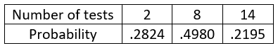
The probability distribution of Y can therefore be represented in this table:

g) Determine the expected value of Y.

This calculation is straightforward: E(Y) = 2(.2824) + 8(.4980) + 14(.2195) ≈ 7.62 tests.

h) Write a sentence or two summarizing your findings, with regard to an optimal plan for minimizing how many tests will be needed in the long run.

Students who correctly determined the expected values realize that the best of these three plans is Plan C.  If this procedure is applied for a very large number of groups, then Plan C will result in an average of about 7.62 tests per group of 12 people.  This is smaller than the average number of tests needed with Plan B (9.61) or Plan A (12.00).

---

Now comes the key question that I did not address in my earlier post about batch testing: Can we do even better (in terms of minimizing the average number of tests needed in the long run) than using 2 sub-groups of 6 people?  I chose the number 12 here on purpose, because it lends itself to several more possibilities: 3 sub-groups of 4, four sub-groups of 3, and six sub-groups of 2.

We can imagine groans emanating from our students at this prospect.  But we can deliver them some good news: We do not need to determine the probability distributions for the number of tests in all of these situations.  We can save ourselves a lot of bother by solving one general case and then using properties of expected values.

i) Let W represent the number of tests needed when an arbitrary number of people (n) are to be tested in a batch.  Determine the probability distribution of W and expected value of W, as a function of n.

The possible values are simply 1 and (n + 1).  We can calculate Pr(W = 1) = Pr(nobody has the disease) = .9ⁿ.  Similarly, Pr(W = n + 1) = Pr(at least one person has the disease) = 1 – .9ⁿ.  The expected value is therefore: E(W) = (1 × .9ⁿ) + (n + 1) × (1 – .9ⁿ) = n + 1 – n(.9ⁿ).  This holds when n ≥ 2.

j) Confirm that this general expression gives the correct expected value for n = 12 people.

I encourage my students to look for ways to check their work throughout a complicated process. Plugging in n = 12 gives: E(W) = 12 + 1 – 12(.9¹²) ≈ 9.61 tests. Happily, this is the same value that we determined earlier.

k) Use the general expression to determine the expected value of the number of tests with a batch of n = 6 people. 

This gives: E(W) = 6 + 1 – 6(.9⁶) ≈ 3.81 tests

l) How does this compare to the expected value for plan C (dividing the group of 12 people into two sub-groups of 6) above?  Explain why this makes sense.

This question holds the key to our short-cut. This expected value of 3.81 is equal to one-half of the expected number of tests with plan C, which was 7.62 tests.  This is not a fluke, because we can express Y (the total number of tests with two sub-groups of 6) as Y = Y₁ + Y₂, where Y₁ is the number of tests with the first sub-group of 6 people, and Y₂ is the number of tests with the second sub-group of 6 people.  Properties of expected value then establish that E(Y₁ + Y₂) = E(Y₁) + E(Y₂).

This same idea will work, and save us considerable time and effort, for all of the other sub-group possibilities that we mentioned earlier.

m) Determine the expected value of the number of tests for three additional plans: three sub-groups of 4 people each, four sub-groups of 3 people each, and six sub-groups of 2 people each.  [Hint: Use the general expression and properties of expected value.]

With a sub-group of 4 people, the expected number of tests with one sub-group is: 4 + 1 – 4(.9⁴) ≈ 2.3756.  The expected value of the number of tests with three sub-groups of 4 people is therefore: 3(2.3756) ≈ 7.13 tests.

With a sub-group of 3 people, the expected number of tests with one sub-group is: 3 + 1 – 3(.9³) ≈ 1.813.  The expected value of the number of tests with four sub-groups of 3 people is therefore: 4(1.813) ≈ 7.25 tests.

With a sub-group of 2 people, the expected number of tests with one sub-group is: 2 + 1 – 2(.9²) = 1.38.  The expected value of the number of tests with six sub-groups of 2 people is therefore: 6(1.38) = 8.28 tests.

n) Write a paragraph to summarize your findings about the optimal sub-group composition for batch-testing in this situation.

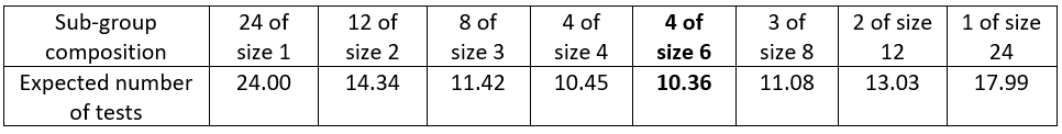
The following table summarizes our findings about expected values:

With a group of 12 people, assuming independence and a disease probability of 0.1 per person, the optimal sub-group composition is to have 3 sub-groups of size 4 people each.  This produces an expected value of 7.13 for the number of tests to be performed.  This is 39.6% fewer tests than the 12 that would have to be conducted without batch testing.  This is also 24.5% fewer tests than would be performed with just one batch.  (See post #28, here, for my pet peeve about misconceptions involving percentage differences.)

---

Let’s conclude with two more extensions of this batch testing problem:

o) How do you predict the optimal sub-group composition to change with a smaller probability that an individual has the disease?  Change the probability to 0.05 and re-calculate the expected values to test your prediction.

It makes sense that larger sub-groups would be more efficient with a more rare disease.  With p = 0.05, we obtain the following expected values for the total number of tests:

In this case with a more rare disease (p = 0.05), the optimal strategy is to divide the 12 people into two groups of 6 people each.  This results in 5.18 tests on average in the long run.

p) How would the optimal sub-group composition change (if at all) if there were twice as many people (24) in the group?

We can simply double the expected values above.  We also have new possibilities to consider: three sub-groups of size 8, and two sub-groups of size 12.  For the p = 0.05 case, this produces the same optimal sub-group size as before, 6 people per sub-group, as shown in the following table of  expected values:

---

Batch testing provides a highly relevant application of expected values for discrete random variables that can also help students to develop problem-solving skills. Speaking of relevance, you may have noticed that COVID-19 and coronavirus did not appear in this post until now.  I did not want to belabor this connection with my students, but I trust that they could not help but recognize the potential applicability of this technique to our current challenges.  I also pointed my students to an interactive feature from the New York Times here, an article in the New York Times here, and an article in Significance magazine here.

P.S. I recorded a video presentation of this batch testing for the College Board, which you can find here.