Posts tagged ‘observational studies’

#44 Confounding, part 2

Many introductory statistics students find the topic of confounding to be one of the most confounding topics in the course.  In the previous post (here), I presented two extended examples that introduce students to this concept and the related principle that association does not imply causation.  Here I will present two more examples that highlight confounding and scope of conclusions.  As always, this post presents many questions for posing to students, which appear in italics.

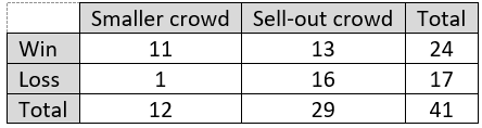
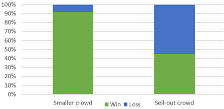
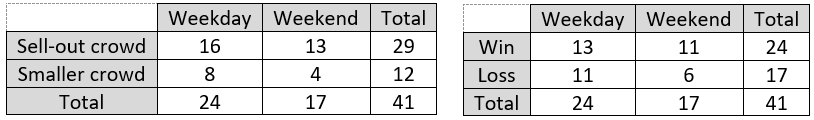
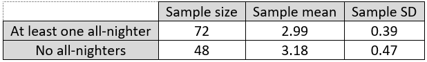
3. A psychology professor at a liberal arts college recruited undergraduate students to participate in a study (here).  Students indicated whether they had engaged in a single night of total sleep deprivation (i.e., “pulling an all-nighter”) during the term.  The professor then compared the grade point averages (GPAs) of students who had and who had not pulled an all-nighter.  She calculated the following statistics and determined that the difference in the group means is statistically significant (p-value < 0.025):

a) Identify the observational units and variables.  What kinds of variables are these?  Which is explanatory, and which is response?

My students know to expect these questions at the outset of every example, to the point that they sometimes groan.  The observational units are the 120 students.  The explanatory variable is whether or not the student pulled at least one all-nighter in the term, which is categorical.  The response variable is the student’s grade point average (GPA), which is numerical.

b) Is this a randomized experiment or an observational study?  Explain how you can tell.

My students realize that this is an observational study, because the students decided for themselves whether to pull an all-nighter.  They were not assigned, randomly or otherwise, to pull an all-nighter or not.

c) Is it appropriate to draw a cause-and-effect conclusion between pulling an all-nighter and having a lower GPA?  Explain why or why not.

Most students give a two-letter answer followed by a two-word explanation here.  The correct answer is no.  Their follow-up explanation can be observational study or confounding variables.  I respond that this explanation is a good start but would be much stronger if it went on to describe a potential confounding variable, ideally with a description of how the confounding variable provides an alternative explanation for the observed association.  The following question asks for this specifically.

d) Identify a (potential) confounding variable in this study.  Describe how it could provide an alternative explanation for why students who pulled an all-nighter have a smaller mean GPA than students who have not.

Students know this context very well, so they are quick to propose many good explanations.  The most common suggestion is that the student’s study skills constitute a confounding variable.  Perhaps students with poor study skills resort to all-nighters, and their low grades are a consequence of their poor study skills rather than the all-nighters.  Another common response is coursework difficulty, the argument being that more difficult coursework forces students to pull all-nighters and also leads to lower grades.  Despite having many good ideas here, some students struggle to express the confounding variable as a variable.  Another common error is to describe the link between their proposed confounding variable and the explanatory variable, neglecting to describe a link with the response.

e) Is it appropriate to rule out a cause-and-effect relationship between pulling an all-nighter and having a lower GPA?  Explain why or why not.

This may seem like a silly question, but I think it’s worth asking.  Some students go too far and think that not drawing a cause-and-effect conclusion is equivalent to drawing a no-cause-and-effect conclusion.  The answer to this question is: Of course not!  It’s quite possible that pulling an all-nighter is harmful to a student’s academic performance, even though we cannot conclude that from this study.

f) Describe how (in principle) you could design a new study to examine whether pulling an all-nighter has a negative impact on academic performance (as measured by grades).

Many students give the answer I’m looking for: Conduct a randomized experiment.  Then I press for more details: What would a randomized experiment involve?  The students in the study would need to be randomly assigned to pull an all-nighter or not. 

g) How would your proposed study control for potential confounding variables? 

I often need to expand on this question to prompt students to respond: How would a randomized experiment account for the fact that some students have better study skills than others, or are more organized than others, or have more time for studying than others?  Some students realize that this is what random assignment achieves.  The purpose of random assignment is to balance out potential confounding variables between the groups.  In principle, students with very good study skills should be balanced out between the all-nighter and no-all-nighter groups, just as students with poor study skills should be similarly balanced out.  The explanatory variable imposed by the researcher should then constitute the only difference between the groups.  Therefore, if the experiment ends up with a significant difference in mean GPAs between the groups, we can attribute that difference to the explanatory variable: whether or not the student pulled an all-nighter.

I end this example there, but you could return to this study later in the course.  You could ask students to conduct a significance test to compare the two groups and calculate a confidence interval for the difference in population means.  At that point, I strongly recommend asking about causation once again.  Some students seem to think that inference procedures overcome concerns from earlier in the course about confounding variables.  I think we do our students a valuable service by reminding them* about issues such as confounding even after they have moved on to study statistical inference. .

* Even better than reminding them is asking questions that prompt students to remind you about these issues.

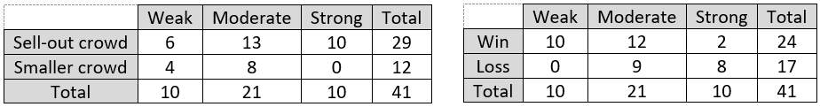
4. Researchers interviewed parents of 479 children who were seen at a university pediatric ophthalmology clinic.  They asked parents whether the child slept primarily in room light, darkness, or with a night light before age 2.  They also asked about the child’s eyesight diagnosis (near-sighted, far-sighted, or normal vision) from their most recent examination. 

a) What are the observational units and variables in this study?  Which is explanatory, and which is response?  What kind of variables are they?

You knew this question was coming first, right?  The observational units are the 479 children.  The explanatory variable is the amount of lighting in the child’s room before age 2.  The response variable is the child’s eyesight diagnosis.  Both variables are categorical, but neither is binary.

b) Is this an observational study or a randomized experiment?  Explain how you can tell.

Students also know to expect this question at this point.  This is an observational study.  Researchers did not assign the children to the amount of light in their rooms.  They merely recorded this information.

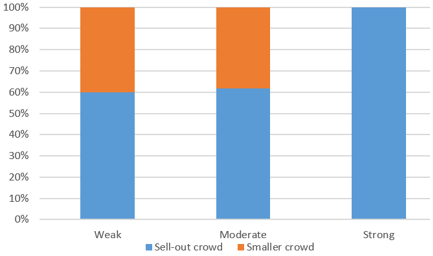
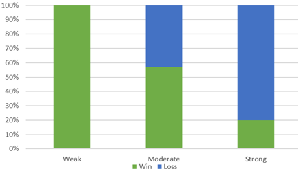
The article describing this study (here) included a graph similar to this:

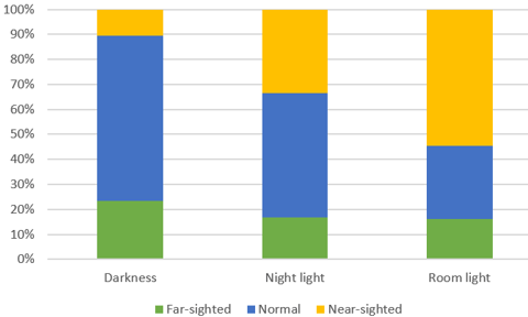
c) Does the graph reveal an association between amount of lighting and eyesight diagnosis?  If so, describe the association.

Yes, the percentage of children who are near-sighted increases as the amount of lighting increases.  Among children who slept in darkness, about 10% were near-sighted, compared to about 34% among those who slept with a night light and about 55% among those who slept with room light.  On the other hand, the percentage with normal vision decreases as the amount of light increases, from approximately 65% to 50% to 30%.

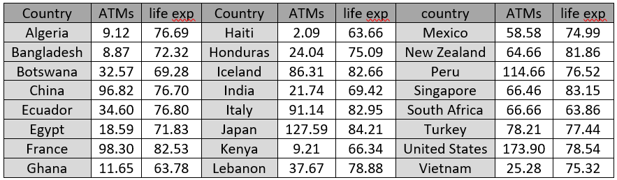
Here is the two-way table of counts:

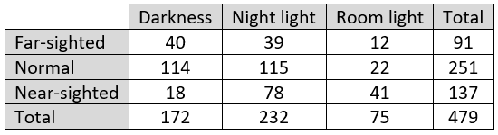
d) Were most children who slept in room light near-sighted?  Did most near-sighted children sleep in room light?  For each of these questions, provide a calculation to support your answer. 

Some students struggle to recognize how these questions differ.  The answer is yes to the first question, because 41/75 ≈ 0.547 of those who slept in room light were near-sighted.  For the second question, the answer is no, because only 41/137 ≈ 0.299 of those who were near-sighted slept in room light.

e) Is it appropriate to conclude that light in a child’s room causes near-sightedness?  Explain your answer. 

No.  Some students reflexively say observational study for their explanation.  Others simply say confounding variables.  These responses are fine, as far as they go, but the next question prompts students to think harder and explain more fully.

f) Some have proposed that parents’ eyesight might be a confounding variable in this study.  How would that explain the observed association between the bedroom lighting condition and the child’s eyesight? 

Asking about this specific confounding variable frees students to concentrate on how to explain the confounding.  Most students point out that eyesight is hereditary, so near-sighted parents tend to have near-sighted children.  Unfortunately, many students stop there.  But this falls short of explaining the observed association, because it says nothing about the lighting in the child’s room.  Completing the explanation requires adding that near-sighted parents may tend to use more light in the child’s room than other parents, perhaps so they can more easily check on the child during the night.

The next set of questions continues this example by asking about how one could (potentially) draw a cause-and-effect conclusion on this topic.

g) What would conducting a randomized experiment to study this issue entail?

Children would need to be randomly assigned to have a certain amount of light (none, night light, or full room light) in their bedroom before the age of 2.

h) How would a randomized experiment control for parents’ eyesight? 

This question tries to help students focus on the goal of random assignment: to balance out all other characteristics of the children among the three groups.  For example, children with near-sighted parents should be (approximately) distributed equally among the three groups, as should children of far-sighted parents and children of parents with normal vision.  Even better, we also expect random assignment to balance out factors that we might not think of in advance, or might not be able to observe or measure, that might be related to the child’s eyesight.

i) What would be the advantage of conducting a randomized experiment to study this issue?

If data from a randomized experiment show strong evidence of an association between a child’s bedroom light and near-sightedness, then we can legitimately conclude that the light causes an increased likelihood of near-sightedness.  This cause-and-effect conclusion would be warranted because random assignment would (in principle) account for other potential explanations.

j) Would conducting such a randomized experiment be feasible in this situation?  Would it be ethical?

To make this feasible, parents would need to be recruited who would agree to allow random assignment to determine how much light (if any) to use in their child’s bedroom.  It might be hard to recruit parents who would give up this control over their child’s environment.  This experiment would be ethical as long as parents were fully informed and consented to this agreement.

You can return to this example, and the observational data from above, later in the course to give students practice with conducting a chi-square test.  This provides another opportunity to ask them about the scope of conclusions they can draw.

l) Conduct a chi-square test.  Report the test statistic and p-value.  Summarize your conclusion.  The test statistic turns out to be approximately 56.5.  With 4 degrees of freedom, the p-value is extremely close to zero, about 7.6×10^(-12).  The data provide overwhelming evidence against the null hypothesis of no association, in favor of the alternative that there is an association between amount of light in the child’s room before age 2 and eyesight diagnosis later in childhood.

m) In light of the very large test statistic and extremely small p-value, is it reasonable to conclude that light in a child’s room causes an increased chance of the child becoming near-sighted?  I think it’s very important to ask this again after conducting the hypothesis test.  Some students mistakenly think that hypothesis tests are so advanced that they can override what they learned earlier in the course.  The extremely small p-value in no way compensates for the observational nature of these data and the possibility of confounding variables.  A cause-and-effect conclusion between bedroom light and near-sightedness still cannot be drawn.

n) Why do you think the researchers bothered to collect and analyze these data, considering that no causal conclusion can be drawn?

Some students believe that a cause-and-effect conclusion is the only kind worth drawing. I ask this question to help them realize that establishing evidence of association can be a worthy goal in its own right, apart from the question of causation.

o) Is it reasonable to generalize this study’s finding about an association between room lighting and near-sightedness to the population of all children in the United States?  Explain.

Most students realize that the correct answer is no, but many mistakenly attribute this to the observational nature of the data.  With regard to generalizability, the key point is that the children in this study were not randomly selected from any population.  They were all patients at a university pediatric ophthalmology clinic, so they are not likely to be representative of all U.S. children with regard to issues involving eyesight.  The finding of an association between increased bedroom light and near-sightedness may or may not hold in the larger population of U.S. children in general.

Asking this question can help students who confuse bias and confounding, or who believe that bias and confounding are the same idea.  This can also remind students of the important distinction between random sampling and random assignment, which I discussed in posts #19 and #20 (Lincoln and Mandela, here and here).

Observational studies abound in many fields.  They often produce intriguing results that are discussed in news media.  Accordingly, it’s important for students to understand the topic of confounding and especially how confounding affects the scope of conclusions that can be drawn from observational studies.  The four examples in this two-part series introduce students to these ideas.  They also provide an opportunity to make connections among different parts of the course, spanning topics of data exploration and statistical inference as well as design of studies and scope of conclusions.

P.S. The topic of drawing cause-and-effect conclusions legitimately from observational studies has become widely studied.  I confess that I do not address this topic in my introductory statistics courses, but some argue strongly that I am doing my students a disservice in this regard.  After all, the most important causal conclusion of the twentieth century may have been that smoking causes cancer, which was not determined by randomly assigning humans to smoke or not.

One of the most prominent advocates for causal inference is Judea Pearl, who has co-authored a general-audience book titled The Book of Why: The New Science of Cause and Effect (information and excerpts can be found here).  Statistics educators who argue for including this topic prominently include Milo Schield (here), Danny Kaplan (here), and Jeff Witmer (here).  A recent article in the Journal of Statistics Education by Cummiskey et al (here) also makes this case.

P.P.S. for teachers of AP Statistics: I’ll be conducting some one-hour sessions via zoom in which I lead students through the first five questions on the 2011 exam, discussing what graders looked for and highlighting common student errors.  I hope this provides some helpful practice and preparation for the upcoming 2020 AP Statistics exam.  Please contact me (allanjrossman@gmail.com) if you would like to invite your students to attend one of these sessions.