#20 Lincoln and Mandela, part 2

In last week’s post (here) I discussed sampling bias and random sampling with an activity that made use of Lincoln’s Gettysburg Address.  Now I present an activity using random assignment that mentions another great leader: Nelson Mandela.

---

This activity starts by asking students to answer two questions about Mandela.  Unbeknownst to my students, I distribute two versions of the questions:

• Version A:
  • Was Nelson Mandela, first president of South Africa following apartheid, younger or older than 16 years old when he died?
  • Make a guess for Mandela’s age when he died.
• Version B:
  • Was Nelson Mandela, first president of South Africa following apartheid, younger or older than 160 years old when he died?
  • Make a guess for Mandela’s age when he died.

Did you notice the subtle difference between the two versions?  They are identical except for one occurrence of the 0 character.  Version A asks about an age of 16, and version B asks about an age of 160.  Both of these questions are ridiculous; everyone knows that Mandela was older than 16 and younger than 160 when he died.  Why ask these silly questions at all?  The research question here is whether people’s age guesses are subconsciously affected by first seeing the number 16 or 160.  The psychological phenomenon known as anchoring suggests that those numbers, despite being completely irrelevant, nevertheless affect subsequent responses.

How do I present these questions to students?  Sometimes I prepare and distribute strips of paper in class, with the two versions mixed up randomly beforehand.  At other times I distribute the questions to students electronically, using either a google form or our course management system.  In this latter case I post both versions and ask students to determine which version to answer by adding the year, date, and month (as a number) of their birthdate. I tell them to use version A if this sum is odd and version B if this sum is even.

---

After we’ve collected students’ responses, I reveal the two versions to students and describe the research question.  Then I ask:

• (a) What are the observational units?  This one is easy: The students themselves are the observational units, because the data were collected on them.
• (b) What are the variables?  Which is explanatory, and which is response?  Classify each variable as categorical or numerical.  This one takes some thought.  The answer to the first question on the survey (older or younger than …) is actually not relevant here.  The explanatory variable is which “anchor” value the student was given: 16 or 160.  This is a categorical (and binary) variable.  The response variable is the guess for Mandela’s age when he died, which is numerical.
• (c) Is this an observational study or an experiment?  This is an experiment, because the explanatory variable groups (i.e., whether a student read the question with 16 or 160 as the anchor value) were actively imposed on the students, not passively observed.  Thinking about the explanatory variable is key here, because some students are tempted to respond that this is an observational study because it feels like only answering survey questions.
• (d) Did this study make use of random sampling, random assignment, both, or neither?  This is an important question, because one of my primary goals with this activity is to reinforce that random sampling and random assignment have different goals and benefits.  I advise students to take this one question at a time:
  • Did we make use of random sampling?  After some time for thought, I often ask a follow-up question as a hint: Who constitutes the sample, and did we choose these people randomly?  Students realize that they comprise the sample.  They were not selected randomly from the population of all students at our university (or from any other population), because they’re all students in my class.
  • Did we make use of random assignment?  Again I provide a hint after allowing some time to think about this: How did students come to be in group A or group B?  Students recognize that they were randomly assigned to a group.
• (e) Some students know more about world history than others.  Is this a confounding variable here?  If not, how was this variable (knowledge of world history) controlled for?  This is a tough question for many students.  But this is a key question that gets at the purpose of random assignment.  The answer is no, this is not a confounding variable, because random assignment should have balanced out those who know lots of world history (or a moderate amount, or not much at all) between the two groups.  That’s what random assignment is all about: creating groups that are as similar as possible in all respects, except for the explanatory variable being studied.
• (f) If it turns out that the age guesses in group B are statistically significantly greater than the age guesses in group A, would it be appropriate to draw a cause-and-effect conclusion?  If so, between what and what?  This is the other key question, as it addresses the scope of conclusion that can potentially be drawn from a randomized experiment.  Because students were randomly assigned to one value or the other for the anchor, it would be legitimate to draw a cause-and-effect conclusion if the age guesses differ significantly, in the conjectured direction, between the two groups.  In other words, it would be appropriate to conclude that the value of the anchor had an effect on these students’ age guesses.

---

I often end this activity there, keeping students’ atention solely on data collection issues.  But you could extend the activity further, or come back to it later in the course, by asking students to analyze and draw conclusions from their data:

• (g) Produce appropriate graphs and calculate relevant statistics.  Summarize what these reveal about the research question.
• (h) Conduct a test to assess the strength of evidence that the data provide for the research hypothesis.  Also calculate and interpret an appropriate confidence interval for comparing the two groups.

Here are results from a recent class of mine, analyzed with Minitab statistical software:

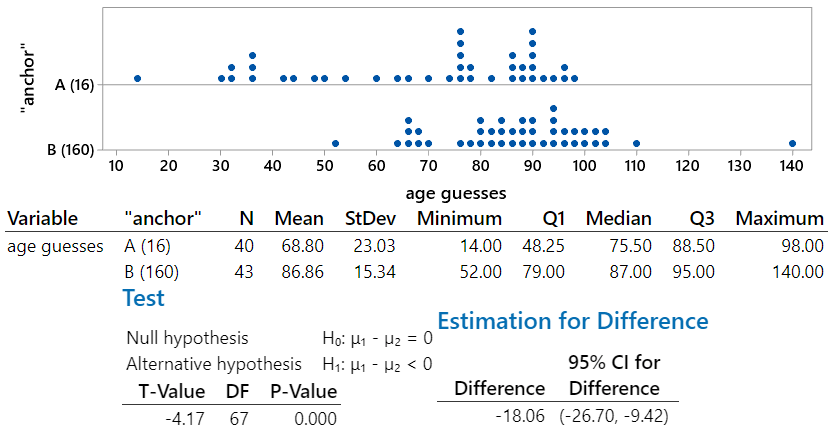
This analysis reveals that the sample data provide strong evidence to support the anchoring phenomenon.  The mean age guesses differ by almost 18 years (68.80 for version A, 86.86 for version B) in the conjectured direction.  The medians, which are not affected by outliers, differ by 11.5 years (75.5 for version A, 87.0 for version B).  The p-value for the t-test comparing the group means is essentially zero, indicating that the class data provide strong evidence to support the hypothesis that responses are affected by the “anchor” number that they see first.  We can be 95% confident that those who see an anchor of 160 produce an average age guess that is between 9.4 and 26.7 years greater than those who see an anchor of 16.

---

These data also provide a good opportunity to ask about whether any values should be removed from the analysis.  Many students believe that outliers should always be discarded, but it’s important to consider whether there is ample justification for removing them. In this case the age guesses of 14 years in group A and 140 years in group B are so implausible as to suggest that the students who gave those responses did not understand the question, or perhaps did not take the question seriously.  Let’s re-analyze the data without those values.  But first let’s ask students to think through what will happen:

• (i) Predict the effect of removing the two extreme data values on:
  • Mean age guess in each group,
  • Standard deviations of the age guesses in each group,
  • Value of the t-test statistic
  • p-value
  • Confidence interval for the difference in population means
• (j) Remove these two data values, and re-analyze the data.  Comment on how (if at all) these quantities change.  Also re-summarize your conclusions, and comment on how (if at all) they change.

After removing the two extreme data values, we produce the following output:

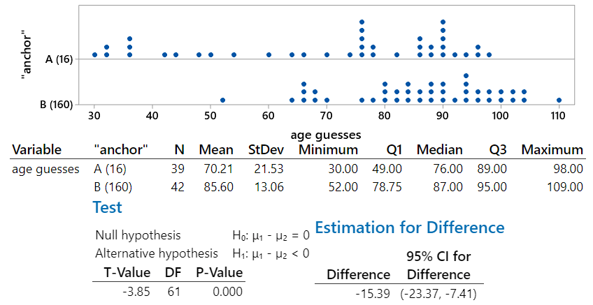
We see that even without the extreme data values, the data still provide strong evidence for the anchoring phenomenon.  As most students will have predicted, the mean age guess increased in version A and decreased in version B.  The standard deviations of the age guesses decreased in both groups.  The smaller difference in group means would move the t-value toward zero, but the smaller within-group standard deviations would produce a larger (in absolute value) t-statistic.  The net effect here is that the value of the t-statistic is slightly less negative. The p-value is the same as before to three decimal places (0.000) but is actually a tad larger due to the smaller (in absolute value) t-statistic.  Similarly, the confidence interval is centered on a smaller difference and is a bit narrower.  Without the extreme data values, we are 95% confident that the average age guess with the 160 anchor is between 7.4 and 23.4 years larger than with the 16 anchor.

---

Before concluding this analysis, I think it’s important to return to two key questions that get at the heart of the different purposes of random sampling and random assignment:

• (k) Is it appropriate to draw a cause-and-effect conclusion from these data?  Justify your answer, and state the conclusion in context.
• (l) To what population is it reasonable to generalize the results of this study?  Justify your answer.

Yes, it is appropriate to draw a cause-and-effect conclusion that the larger anchor number tends to produce greater age guesses than the smaller anchor number.  This conclusion is warranted, because the study design made use of random assignment and the resulting data revealed a highly statistically significant difference in the average age guesses of the two groups.

But this study only included students from my class, which is not a random sample from any population.  We should be careful not to generalize this conclusion too broadly.  Perhaps other students at my university would react similarly, and perhaps students in general would respond similarly, but we do not have data to address that.

---

I mentioned in post #11, titled “Repeat after me” (here), that I ask questions about observational units and variables over and over in almost every example throughout the entire course.  After we’ve studied random sampling and random assignment, I also ask questions about this, like questions (c) and (d) above, for virtually every example.  I also ask questions about scope of conclusions, like questions (k) and (l) above, for almost every example also.

To assess students’ understanding of the distinction between random sampling and random assignment, I also ask questions such as:

• You want to collect data to investigate whether teenagers in the United States have read fewer Harry Potter books (from the original series of seven books) than teenagers in the United Kingdom.  Would you make use of random sampling, random assignment, both, or neither?  Explain.
• An instructor wants to investigate whether using a red pen to grade assignments leads to lower scores on exams than using a blue pen to grade assignments.  Would you advise the professor to make use of random sampling, random assignment, both, or neither?  Explain.
• A student decides to investigate whether NFL football games played in indoor stadiums tend to have more points scored than games played outdoors.  The student examines points scored in every NFL game of the 2019 season. Has the student used random sampling, random assignment, both, or neither?

The Harry Potter question cannot involve random assignment, because it makes no sense to randomly assign teenagers to live in either the U.S. or U.K.  But it would be good to use random sampling to select the teenagers in each country to be asked about their Harry Potter reading habits.  On the other hand, it’s important to use random assignment for the question about red vs. blue pen, because the research question asks for a cause-and-effect conclusion.  It’s less important to select a random sample of the instructor’s students, and the instructor would probably want to include all of his or her students who agreed to participate in the study.  For the football question, the student investigator would use neither random assignment nor random sampling.  NFL games are not assigned at random to be played in an indoor stadium or outdoors, and the games from the 2019 season do not constitute a random sample from any population.

---

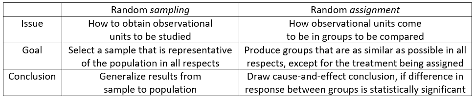
The Lincoln and Mandela activities aim to help students understand that despite the common word random, there’s actually a world of difference between random sampling and random assignment:

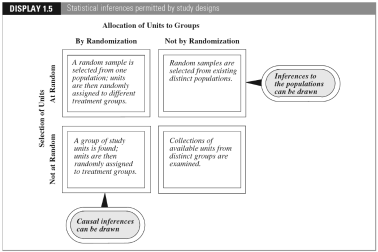
The textbook titled The Statistical Sleuth, by Fred Ramsey and Dan Schafer, presents the following graphic, illustrating the different scopes of conclusions that can be drawn from a statistical study, depending on whether random sampling and/or random assignment were employed:

I recommend emphasizing this distinction between random sampling and random assignment at every opportunity.  I also think we do our students a favor by inviting Lincoln and Mandela into our statistics courses for a brief visit.

---

P.S. Nelson Mandela (1918 – 2013) was 95 years old when he died. You can read about the anchoring phenomenon here, and an article about using the effect of implausible anchors appears here.  The data on age guesses used above can be found in the Excel file below.