#18 What do you expect?

I argued in post #6 (here) that the most dreaded two-word term in statistics is standard deviation.  In this post I discuss the most misleading two-word term in statistics.  There’s no doubt in my mind about which term holds this distinction.  What do you expect me to say?

If you expect me to say expected value, then your expectation is correct.

Below are four examples for helping students to understand the concept of expected value and avoid being misled by its regrettable name.  You’ll notice that I do not even use that misleading name until the end of the second example.  As always, questions that I pose to students appear in italics.

---

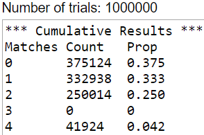
1. Let’s return to the random babies activity from post #17 (here).  I used the applet (here) to generate one million repetitions of distributing four babies to their mothers at random, with the following results:

I ask students: Calculate the average number of matches per repetition.  I usually get some blank stares, so I ask: Remind me how to calculate an average.  A student says to add up the values and then divide by the number of values.  I respond: Yes, that’s all there is to it, so please do that with these one million values.  At this point the blank stares resume, along with mutterings that they can’t possibly be expected* to add a million values on their own.

* There’s that word again.

But of course adding these one million values is not so hard at all: Adding the 375,124 zeroes takes no time, and then adding the 332,938 ones takes barely a moment.  Then you can make use of a wonderful process known as multiplication to calculate the entire sum: 0×(375,124) + 1×(332,938) + 2×(250,014) + 4×(41,924) = 1,000,662.  Dividing by 1,000,000 just involves moving the decimal point six places to the left.  This gives 1.000662 as the average number of matches in the one million simulated repetitions of this random process of distributing four babies to their mothers at random.

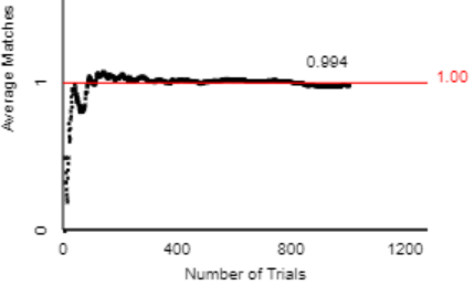
Then I ask: What do you think the long-run average (number of matches per repetition) will be if we continue to repeat this random process forever and ever?   Most students predict that the long-run average will be 1.0, and I tell them that this is exactly right.  I also show the applet’s graph of the average number of matches as a function of number of repetitions (for the first 1000 repetitions), which shows considerable variation at first but then gradual convergence toward a long-run value:

---

At this point we discuss how to calculate the theoretical long-run average based on exact probabilities rather than simulation results.  To derive the formula, let’s rewrite the calculation of the average number of matches in one million repetitions from above:

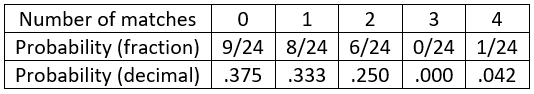
Notice that this calculation is a weighted average, where each possible value (0, 1, 2, 4) is weighted by the proportion of repetitions that produced the value.  Now recall the exact probabilities that we calculated in post #17 (here) for this random process:

and then replace the proportions in the weighted average calculation with the exact, theoretical probabilities:

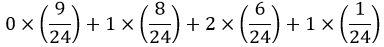
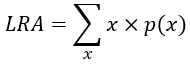
This expression works out to be 24/24, which is better known as the value 1.0.  This is the theoretical long-run average number of matches that would result from repeating this random process forever and ever.  In general, a theoretical long-run average is the weighted average of the possible values of the random process, using probabilities as weights.  We can express this in a formula as follows, where LRA represents long-run average, x represents the possible values, and p(x) represents their probabilities:

Back to the random babies context, next I ask:

• Is this long-run average the most likely value to occur?  Students recognize that the answer is no, because we are slightly more likely to obtain 0 matches than 1 match (because probability 9/24 is greater than 8/24).
• How likely is the long-run average value to occur?  We would obtain exactly 1 match one-third (about 33.33%) of the time, if we were to repeat the random process over and over.
• Do you expect the long-run average value to occur if you conduct the random babies process once?  Not really, because it’s twice as likely that we will not obtain 1 match than it is that we will obtain 1 match.

---

2. Now a very generic example: Consider rolling a fair, ordinary, six-sided die (or number cube), and then observing the number of dots on the side that lands up.  Calculate and interpret the long-run average value from this random process.

Saying that the die is fair means that the six possible outcomes should be equally likely, so the possible values and their probabilities are:

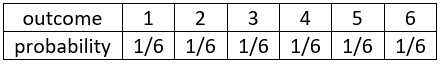
We can calculate the long-run average to be: LRA = 1×(1/6) + 2×(1/6) + 3×(1/6) + 4×(1/6) + 5×(1/6) + 6×(1/6) = 21/6 = 3.5.  This means that if we were to roll the die for a very large number of rolls, the average number of dots appearing on the side that lands up would be very close to 3.5.

Now I ask the same three questions from the end of the previous example:

• Is this long-run average the most likely value to occur in the die-rolling process?  Of course not, because it’s downright impossible to obtain 3.5 dots when rolling a die. 
• How likely is the long-run average value to occur?  Duh, like I just said, it’s impossible!  The probability is zero.
• Do you expect the long-run average value to occur if you roll a die once?  Once more, with feeling: Of course not!

Students naturally wonder why I asked these seemingly pointless questions for the die-rolling example.  Here’s where things get a bit dicey (pun intended).  I sheepishly reveal to students that the common term for this quantity that we have been calculating and interpreting is expected value, abbreviated as EV or E(X).

Let’s ask those questions again about the die-rolling process, but now using standard terminology:

• Is the expected value the most likely value to occur in the die-rolling process? 
• How likely is the expected value to occur? 
• Do you expect the expected value to occur if you conduct the die rolling process once? 

The answers to these questions are the same as before: No, of course not, the expected value (3.5 dots) is certainly not expected, because it’s impossible!

Isn’t this ridiculous?  Can we blame students for getting confused between the expected value and what we expect to happen?  As long as we’re stuck with this horribly misleading term, it’s incumbent on us to help students understand that the expected value of a random process does not in any way, shape, or form mean the value that we expect to occur when we conduct the random process.  How can we do this?  You already know my answer: Ask good questions!

---

3. Now let’s consider the gambling game of roulette.  When an American roulette wheel (as shown below) is spun, a ball eventually comes to rest in one of its 38 numbered slots.  The slots have colors: 18 red, 18 black, and 2 green.

The simplest version of the game is that you can bet on either a number or a color:

• If you bet $1 on a color (red or black) and the ball lands in a slot of that color, then you get $2 back for a net profit of $1.  Otherwise, your net profit is -$1.
• If you bet $1 on a number and the ball lands in that number’s slot, then you get $36 back for a net profit of $35.  Otherwise, your net profit is -$1.

I ask students to work through the following questions in groups, and then we discuss the answers:

• a) List the possible values of your net profit from a $1 bet on a color, and also report their associated probabilities.  The possible values for net profit are +1 (if the ball lands on your color) and -1 (if it lands on a different color).  The wheel contains 18 slots of your color, so the probability that your net profit is +1 is 18/38, which is about 0.474.  The probability that your net profit is -1 is therefore 20/38, which is about 0.526.  Not surprisingly, it’s a little more likely that you’ll lose than win.
• b) Determine the expected value of the net profit from betting $1 on a color.  The expected value is $1×(18/38) + (-$1)×(20/38) = -$2/38, which is about -$0.053.
• c) Interpret what this expected value means.  If you were to bet $1 on a color for a large number of spins of the wheel, then your average net profit would be very close to a loss of $0.053 (about a nickel) per spin.
• d) Repeat (a)-(c) for betting $1 on a number.  The possible values of net profit are now +35 (if the balls lands on your number) and -1 (otherwise).  The respective probabilities are 1/38 (about 0.026) and 37/38 (about 0.974).  The expected value of net profit is $35×(1/38) + (-$1)×(37/38) = -$2/38, which is about -$0.053.  If you were to bet $1 on a number for a large number of spins of the wheel, then your average net profit would be very close to a loss of $0.053 (about a nickel) per spin.
• e) How do the expected values of the two types of bets compare?  Explain what this means.  The two expected values are identical.  This means that if you bet for a large number of spins, your average net profit will be to lose about a nickel per spin, regardless of whether you bet on a color or number.
• f) Are the two types of bets identical?  (Would you get the same experience by betting on a color all evening vs. betting on a number all evening?)  If not, explain their primary difference.  No, the bets are certainly not identical, even though their expected values are the same.  If you bet on a number, you will win much less often than if you bet on a color, but your winning amount will be much larger when you do win.
• g) The expected value from a $1 bet might seem too small to form the basis for the huge gambling industry.  Explain how casinos can make substantial profits based on this expected value.  Remember that the expected value is the average net profit per dollar bet per spin.  Casinos rely on attracting many customers and keeping them gambling for a large number of spins.  For example, if 1000 gamblers make $1 bets on 1000 spins each, then the expected value* of the casino’s income would 1000×1000×($2/38) ≈ $52,638.58.

* I have resisted the temptation to use a shorthand term such as expected income or expected profit throughout this example.  I believe that saying expected value every time might help students to avoid thinking of “expected” in the everyday sense of the word when we intend its technical meaning.

---

4. I like to use this question on exams to assess students’ understanding of expected value: At her birthday party, Sofia swings at a piñata repeatedly until she breaks it.  Her mother tells Sofia that she has determined the probabilities associated with the possible number of swings that could be needed for Sofia to break the piñata, and she has calculated the expected value to be 2.4.  Interpret what this expected value means.

A good answer is: If Sofia were to repeat this random process (of swinging until she breaks a piñata) for a very large number of piñatas, then the long-run average number of swings that she would need will be very close to 2.4 swings per piñata.

I look for three components when grading students’ interpretations: 1) long-run, 2) average, and 3) context.  Let’s consider each of these:

1. The phrase long-run does not need to appear, but the idea of repeating the random process over and over for a large number of repetitions is essential.  I strongly prefer that the interpretation describe what “long run” means by indicating what would be repeated over and over (in this case, the process of swinging at a piñata until it breaks).  
2. The idea of “average” is absolutely crucial to interpreting expected value, but it’s not uncommon for students to omit this word from their interpretations.   The interpretation makes no sense if it says that Sofia will take 2.4 swings in the long run.
3. As is so often the case in statistics, context is key.  If a student interprets the expected value as “long-run average” with no other words provided, then the student has not demonstrated an ability to apply the concept to this situation.  In fact, a student could respond “long-run average” without bothering to read a single word about the context.

I also think it’s helpful to ask students, especially those who are studying to become teachers themselves, to critique hypothetical responses to interpreting the expected value, such as:

• A. The long-run average is 2.4 swings.
• B. The average number of swings that Sofia needs to break the piñata is 2.4 swings.
• C. If Sofia were to repeat this random process (of swinging until she breaks a piñata) for a very large number of piñatas, then she would need very close to 2.4 swings in the long run.

I would assign partial credit to all three of these responses. Response A is certainly succinct, and it includes the all-important long-run average.  But the only mention of context in response A is the word “swings,” which I do not consider sufficient for describing the process of Sofia swinging at a piñata until it breaks.  Response B sounds pretty good, as it mentions average and describes the context well, but it is missing the idea of long-run.  Adding “if she were to repeat this process with a large number of piñatas” to response B would make it worthy of full credit.  Response C is so long and generally on-point that it might be hard to see what’s missing.  But response C makes no mention of the word or idea of average.  All that’s needed for response C to deserve full credit is to add “on average” at the end or insert “an average of” before “2.4 swings.”

---

Can we expect students to understand what expected value means?  Sure, but the unfortunate name makes this more of a challenge than it should be, as it practically begs students to confuse expected value with the value that we expect to occur.  As much as I would like to replace this nettlesome term with long-run average and its abbreviation LRA, I don’t expect* this alternative to catch on in the short term.  But I do hope that this change catches on before the long run arrives.

* Sorry, I can’t stop using this word!

P.S. I borrowed the scenario of Sofia swinging at a piñata from my colleague John Walker, who proposed this context in an exam question with more involved probability calculations.