#36 Nearly normal

Some students mistakenly believe that everything follows a normal* distribution.  Much closer to the truth is that nothing follows a normal distribution.  George Box famously said: All models are wrong; some models are useful.  The normal distribution provides a useful model for the pattern of variation in many numerical variables.  It also provides a valuable model for how many sample statistics vary, under repeated random sampling from a population.

* This normal word is not quite as objectionable and misleading as expected value (see post #18 here), but it’s still an unfortunate term.  I try to convince students that so-called normal distributions are not all that normal in any sense, and they certainly do not provide the inevitable shape for the distribution of all, or even most, numerical variables.  I realize that I could use the term Gaussian distribution, but that’s too math-y.  Some people capitalize Normal to distinguish the distribution from the everyday word, but that’s quite subtle.  I’d prefer to simply called them bell-shaped distributions, although I know that’s too vague, for example because t-distributions are also bell-shaped.

In this post, I present questions about normal distributions that my students answer in class.  The first is a straightforward introduction to the basics of normal distribution calculations.  The second tries to make clear that a normal distribution is not an appropriate model for all numerical data.  The third asks students to think through how the mean and standard deviation affect a normal distribution in a manufacturing context.  As always, questions that I pose to students appear in italics.

---

I use the context of birthweights to lead students through basic questions involving calculations of probabilities and percentiles from normal distributions.  I like to draw students’ attention to two different wordings for these kinds of questions.  You’ll notice that question (b) asks about a proportion of a population, whereas question (c) asks for a probability involving a randomly selected member of the population.

1. Suppose that birthweights of newborn babies in the United States follow a normal distribution with mean 3300 grams and standard deviation 500 grams.  Babies who weigh less than 2500 grams at birth are classified as low birthweight.

• a) How many standard deviations below the mean is a baby classified as low birthweight?

I realize that calculating a z-score can be considered an unnecessary intermediate step when students are using technology rather than an old-fashioned table of standard normal probabilities.  But I think a z-score provides valuable information*, so I like to start with this question.  Because (2500 – 3300) / 500 = -1.60, a low birthweight baby is at least 1.60 standard deviations below the mean birthweight.

* I discussed z-scores at some length in post #8 (End of the alphabet, here).

Based on the normal model:

• b) What percentage of newborn babies weigh less than 2500 grams? 
• c) What is the probability that a randomly selected newborn baby weighs more than 10 pounds?
• d) What percentage of newborn babies weigh between 3000 and 4000 grams?
• e) How little must a baby weight to be among the lightest 2.5% of all newborns?
• f) How much must a baby weigh to be among the heaviest 10%?

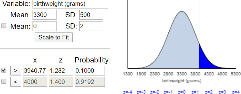
Frankly, I don’t care much about whether students carry out these calculations with an old-fashioned table of standard normal probabilities or with technology.  I give my students access to an old-fashioned table and describe how to use it.  I also show students several choices for using technology (e.g., applet, Minitab, R, Excel).  I always encourage students to start with a well-labeled sketch of a normal curve, with the probability of interest shaded as an area under the normal curve.

The answer to part (b) is that the normal model predicts that 5.48% of newborns are of low birthweight, as shown in this applet (here) output:

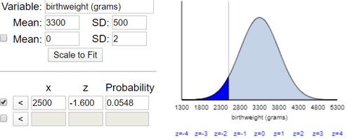
I like that this applet draws a well-labeled sketch with the correct percentage shown as the shaded (dark blue) under the curve.  I also like that the applet reports the z-score as well as the probability. 

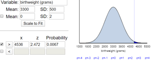
Part (c) requires that students first convert 10 pounds into grams.  They are welcome to use the internet to help with this conversion to approximately 4536 grams.  If they are using a standard table of cumulative probabilities, students must realize that they need to subtract the probability given in the table from one.  The applet reports that this probability that a baby weighs more than ten pounds is only 0.0067, as shown here:

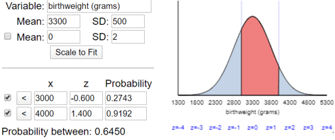
Part (d) requires students to subtract two probabilities if they are using a table.  The applet shows this percentage to be 64.50%, as shown here:

I emphasize to students that parts (e) and (f) ask fundamentally different questions from parts (b)-(d).  The previous parts asked for probabilities from given values; the upcoming parts ask for the birthweight values that produce certain probabilities.  In other words, parts (e) and (f) ask for percentiles, a term with which students are aware but probably need some reinforcement to understand well.

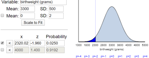
Students can answer part (e) approximately, without a table or software, by remembering the empirical rule.  The cut-off value for the bottom 2.5% of a normal distribution is approximately 2 standard deviations below the mean, which gives 3300 – 2×500 = 2300 grams.  A more precise answer comes from using a z-score of -1.96 rather than -2, which gives 2320 grams, as shown here:

To answer part (f) with a table, students need to realize that the question asks for the 90^th percentile.  The applet shows that this value is approximately 3941 grams:

These questions are quite routine.  The more interesting part comes from thinking about this normal distribution as a model for actual birthweight data.  At this point, I show students this table from the National Vital Statistics Reports (here):

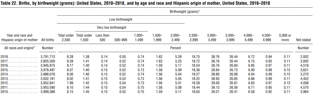
• (g) According to this table, what percentage of newborns in 2018 weighed between 3000 and 3999 grams?  How does this compare with what the normal model predicted in part (d)?

The table reports that 38.76% + 26.44% = 65.20% of newborns weighed between 3000 and 3999 grams, which is very close to the normal model’s prediction of 64.50% from part (d).

• (h) Compare the predictions from the normal model in parts (b) and (c) to the actual counts.

The normal model’s predictions are less good in the tails of the distribution than near the middle.  The normal model predicted that 5.48% would be of low birthweight, but the actual counts show that 8.28% were of low birthweight.  If we use 4500 rather than 4536 for the approximate ten-pound value, we find that 0.94% + 0.11% = 1.05% of newborns weighed more than 4500 grams, compared to a prediction of about 0.67% from the normal model using 4536 grams.

What’s the bottom line here: Do birthweights follow a normal distribution?  Certainly not exactly, but closely enough that the normal model provides a useful approximation.

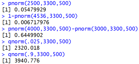
I want students in more mathematical courses to become comfortable with the concept of a cumulative distribution function (cdf).  So, I ask these students to use the pnorm (cdf) and qnorm (inverse cdf) commands in R, in addition to using the more visual applet, to perform these calculations.  The following output shows how to answer parts (b)-(f) with these R commands:

---

2. I recorded the game time (in minutes) until first goal for a sample of 41 National Hockey League games played on October 16-22, 2017.  The distribution of these times is displayed in the following histogram, for which the mean is 11.4 minutes and standard deviation is 10.6 minutes:

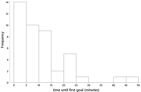
• a) Would it be appropriate to use a normal model for the distribution of times until first goal?  Explain.
• b) If you were to model these times with a normal distribution (using the sample mean and standard deviation), what is the probability that the time until first goal would be negative?
• c) Comment on what the calculation in part (b) indicates about the suitability of using a normal model for time until first goal.

Students recognize immediately that this distribution is highly skewed, not bell-shaped in the least, so a normal model is completely inappropriate here.  The calculation in part (b) produces a z-score of (0 – 11.4) / 10.6 ≈ -1.08 and a probability of 0.141.  This means that a normal model would predict that about 1 in 7 hockey games would have a goal scored before the game began!  This calculation provides further evidence, as if any were needed, that a normal model would be highly inappropriate here.

This example takes only 10 minutes of class time, but I think it’s important to remind students that many numerical variables follow distributions that are not close to normal.  I also like that part (b) gives more practice with a routine calculation, even while the focus is on the inappropriateness of the normal model in this case.

---

The next series of questions asks students to think more carefully about properties of normal curves, particularly how the mean and standard deviation affect the distribution. 

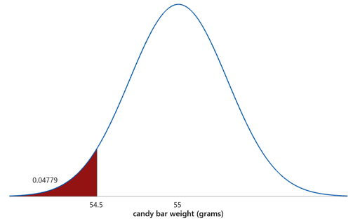
3. Suppose that a candy bar advertises on its wrapper that its weight is 54.5 grams.  The actual weights vary a bit from candy bar to candy bar.  Let’s suppose that the actual weights follow a normal distribution with mean μ = 55.0 grams and standard deviation σ = 0.3 grams.

a) What percentage of candy bars weigh less than advertised?  This is a very routine calculation.  The z-score is -1.67, and the probability is .0478, so 4.78% of candy bars weigh less than advertised, as shown here:

b) Now suppose that the manufacturer wants to reduce this percentage so only 1% of candy bars weigh less than advertised.  If the standard deviation remains at 0.3 grams, would the mean need to increase or decrease?  Explain.  I encourage students to think about this visually: To get a smaller percentage below 54.5 grams, does the mean (and therefore the distribution) need to shift to the right or the left?  Most students realize that the curve needs to shift to the right, so the mean needs to be larger.

c) Determine the value of the mean that would achieve the goal that only 1% of candy bars weigh less than advertised.  Students cannot easily plug given numbers into an applet and press a button to answer this question.  They need to think through how to solve this.  The first step is to determine the z-score for the bottom 1% of a normal distribution, which turns out to be -2.326.  This tells us that the advertised weight (54.5 grams) must be 2.326 standard deviations below the mean.  We can then calculate the mean by adding 2.326 standard deviations to the advertised weight: 54.5 + 2.326 × 0.3 ≈ 55.20 grams.

Normal curves with the original mean (in blue) and the new mean (red dashes) are shown below.  The area to the left of the value 54.5, representing the percentage of candy bars that weigh less than advertised, is smaller with the new mean:

d) What is the downside to the manufacturer of making this change?  I want students to realize that increasing the mean weight means putting more candy in each bar, which will have a cost, perhaps substantial, to the manufacturer.

e) Now suppose that the manufacturer decides to keep the mean at 55.0 grams.  Instead they will change the standard deviation to achieve the goal that only 1% of candy bars weigh less than advertised.  Would the standard deviation need to increase or decrease to achieve this goal?  Explain.  When students need a hint, I ask: Does the original normal curve need to get taller and narrower, or shorter and wider, in order to reduce the area to the left of the value 54.5 grams?  This question is harder than the one about shifting the mean, but most students realize that the curve needs to become taller and narrower, which means that the standard deviation needs to decrease.

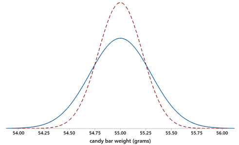
f) Determine the value of the mean that would achieve the goal that only 1% of candy bars weigh less than advertised.  Once again we need a z-score of -2.326 to determine the bottom 1% of the distribution, which again means that the advertised weight needs to be 2.326 standard deviations below the mean.  We can express this algebraically as: (54.5 – 55.0) / σ = -2.326.  Solving gives: σ = (55.0 – 54.5) / 2.326 ≈ 0.215 grams.

Normal curves with the original standard deviation (in blue) and the new one (red dashes) are shown below.  The area to the left of the value 54.5 is smaller with the new standard deviation:

g) Why might this be a difficult change for the manufacturer to make?  Decreasing the standard deviation of the weights requires making the manufacturing process less variable, which means achieving more consistency in the weights from candy bar to candy bar.  Reducing variability in a manufacturing setting can be a daunting task.

h) By what percentage does the manufacturer need to decrease the standard deviation of the weights in order to achieve this goal?  Percentage change is a challenging topic for students, so I look for opportunities to ask about it often*.  The manufacturer would need to decrease the standard deviation of the weights by (0.215 – 0.3) /  0.3 × 100% ≈ 28.3% to achieve this goal.

* See post #28 (A persistent pet peeve, here) for many more examples.

---

Teachers of introductory statistics must decide:

• Whether to teach normal distributions as models for numerical data or only as approximations for sampling distributions;
• Whether to include the process of standardization to z-scores when performing calculations involving normal distributions;
• Whether to ask students to use a table of standard normal probabilities or use only technology for calculating probabilities and percentiles from normal distributions.

You can tell from the examples above that my answers are yes to the first two of these, and I don’t much care about whether students learn to read an old-fashioned normal probability table.  I do care that students learn that a normal curve only provides a model (approximation) for a distribution of real data, and that many numerical variables have a distribution that is not close to normal.  I also expect students to learn how to think carefully through normal distribution calculations that go beyond the basics.

In a follow-up post, I will describe an activity that gives students more practice with normal distribution calculations while also introducing the topic of classification and exploring the concept of trade-offs between different kinds of classification errors.