#50 Which tire?

Perhaps you and your students have heard the campus legend* about two students who miss an exam due to excessive partying, but they tell their professor that they had a flat tire.  They realize that this sounds like a flimsy excuse, so they are pleasantly surprised when the professor accepts their explanation and offers a make-up exam on the following morning.  When they arrive for the make-up exam, they are sent to two separate rooms.  They find question 1, worth 5 points, to be quite straight-forward.  Then they turn the page to find question 2, worth 95 points: Which tire was it?

* I first heard of this story from the “Ask Marilyn” column in the Parade section of the Sunday newspaper on March 3, 1996.  Laurie Snell wrote about this for Chance News (here).  Laurie wrote to the professor involved, a chemist named Dr. Bonk at Duke University.  Dr. Bonk confirmed that something of the sort had happened, but he could not remember the details and suspected that they had been embellished over time.

I ask my students to imagine themselves in this nerve-wracking situation, even though I know that none of them would ever tell a lie to a professor.  I ask them to think about which tire they would say – left front, left rear, right front, or right rear – and write down their answer.  Before I continue with this post, let me ask you to decide on your answer.

Then I predict that one particular tire tends to be selected more often than random chance would expect – the right front tire.  Next we gather data on their response with a simple show of hands.  Telling the story and collecting the data takes less than five minutes of class time.

Here’s the great thing: In addition to getting a laugh from a fun story, you can use these data to introduce or review several topics in an introductory statistics course.  Below I will present and describe six extended exercises, all with different learning objectives, based on this fun and quick data collection exercise.  The topics* of these exercises are:

1. Simulation-based inference
2. Binomial distribution
3. Sample result in opposite direction from conjecture
4. One-proportion z-test and z-interval
5. Impact of sample size on p-value, confidence interval
6. Chi-square goodness-of-fit test

* If you do not have time to read all of these, I recommend #3 and #5 as the least routine.

As always, questions that I pose to students appear in italics.

---

The first exercise uses class data from this activity to practice applying simulation-based inference with a null hypothesis other than 50/50 in which to apply simulation-based inference, unlike the studies on blindsight and facial prototyping (as in post #12 here) and choice of Halloween treats (as in post #13 here).

1. In the spring quarter of 2018, 17 of 44 students in my class selected the right front tire.

• a) Identify the observational units and variable.  Also classify the variable as categorical or numerical.
• b) State (in words) the null and alternative hypotheses to be tested.
• c) Calculate the sample proportion of students who selected the right front tire.
• d) Specify the input values for a simulation analysis to assess the strength of evidence for my claim provided by the data.
• e) Run the simulation analysis, and describe the resulting null distribution of the sample proportion.
• f) Report and interpret the approximate p-value.
• g) Summarize your conclusion, and explain how it follows from the p-value.

As I described in post #11 (Repeat after me, here), I like to ask part (a) repeatedly (as I described in post #Z).  The observational units are students, and the variable is which tire they pick.  This variable is categorical, not binary except that my conjecture treats it as binary.  The null hypothesis is that 25% of all students would pick the right front tire, in other words that there’s nothing special about the right front tire.  The alternative hypothesis is that more than 25% of all students would pick the right front tire, that there’s something special about the right front tire that makes it pop into minds first.  The sample proportion who selected the right front tire is 17/44 ≈ 0.386.

To conduct a simulation analysis, the input values are a success probability of 0.25, sample size of 44, and a large number such as 1000 or 10,000 repetitions.  Using an applet (here) to run this simulation produces an approximate null distribution as shown on the left:

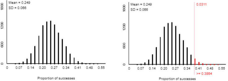
The graph on the right reveals that the approximate p-value is 0.0311.  This means that if students only had a 25% chance of picking the right front tire, then there’s a little more than a 3% chance that 17 or more of 44 students would have picked the right front tire.  Less than 0.05 but greater than 0.01, this is a fairly small, but not very small, p-value.  We conclude that the sample data provide fairly strong, but not very strong, evidence for the theory that students pick the right front tire more than would be expected by random chance.

---

I also use these data to give students experience with recognizing and applying the binomial probability distribution.

2. Let the random variable X represent the number of students in a class of 44 who select the right front tire.  Assume that each student makes their selection independently. Also assume (for now) that each student selects randomly from the four tire options.

• a) Describe the probability distribution of X by giving its name and specifying its parameter values.
• b) Calculate Pr(X ≥ 17).  Feel free to use software or a calculator.  Show how you calculate this.
• c) In the spring quarter of 2018, 17 of 44 students in my class selected the right front tire.  What conclusion would you draw?  Explain how this conclusion follows from the probability in (b).

The probability distribution of X is binomial with parameters n = 44 and p = 0.25.  We can calculate Pr(X ≥ 17) by taking 1 – Pr(X ≤ 16) ≈ 1 – 0.9682 = 0.0318.  This is a fairly small probability, so the observed result would be fairly surprising if the assumption that p = 0.25 were true, so the sample data provide fairly strong evidence that students have a higher probability than 0.25 for selecting the right front tire.

---

The “which tire” in-class data collection activity is not foolproof, in that the sample data does not always turn out as predicted.  But a disappointing result can provide an opportunity for a worthwhile lesson.

3. At a recent workshop for college professors, 8 of 36 workshop participants selected the right front tire.

• a) Explain why it’s not necessary to carry out calculations for a hypothesis test of whether the sample data provide strong evidence that people select the right front tire more often than would be expected by random chance.
• b) Without performing an analysis, what can you say about how the p-value would turn out? 
• c) Based on this sample result, would you reject the null hypothesis?  Explain.
• d) Based on this sample result, would you accept the null hypothesis?  Explain.

Before we jump in to perform a full hypothesis test, I encourage students to look at the sample result: Only 8/36 ≈ 0.222 of the sample selected the right front tire.  This is less than one-fourth, so this is in the wrong direction from our conjecture and the alternative hypothesis.  In light of this, we already know (of course!) that the sample data do not provide strong evidence to suggest that more than one-fourth of all people would select the right front tire.  There’s no need to conduct a formal test to realize and conclude this. 

I think this is a fruitful conversation to have with students, who are often tempted to follow a procedure, or plug into a formula, without thinking things through in advance.

If we were to calculate a p-value here, we know that it would be greater than 0.5.  (In fact, the binomial p-value turns out to be 0.710.)  We certainly do not reject the null hypothesis.  But we also cannot accept the null hypothesis, because there are many other potential values of the parameter than are also consistent with the sample result.

---

I also like to use a larger sample size, by combining results across several classes, to give students practice with applying a one-proportion z-test.

4. In the winter quarter of 2017, 56 of 120 students across my several classes selected the right front tire.

• a) Calculate the proportion of these students who selected the right front tire.  Is this a parameter or a statistic?  Explain.
• b) Write a sentence describing the parameter of interest.
• c) State the null and alternative hypotheses to be tested.
• d) Check whether the sample size conditions for a one-proportion z-test are satisfied.
• e) Calculate and interpret the value of the test statistic.
• f) Summarize your conclusion, and provide justification based on the test statistic.
• g) Calculate and interpret a 95% confidence interval for the parameter.
• h) To what population would you feel comfortable generalizing the results of this analysis?

The proportion who selected the right front tire is 56/120 ≈ 0.467.  This is a statistic, because it’s based on the sample of students in my classes.  The parameter of interest is the proportion of all students at my university who would select the right front tire.  I’m assuming here that the population of interest is all students at my university, but you could also take the population to be a broader group.  Of course, the students in my class were not randomly selected from any population, so we should be cautious about generalizing the results of this analysis.

The null hypothesis is that one-fourth of all students would select the right front tire.  The alternative hypothesis is that more than one-fourth would select the right front tire.  The sample size condition is satisfied because 120×1/4 = 30 and 120×3/4 = 90 are both larger than 10.  The test statistic is:

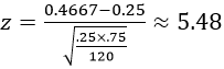
The observed value of the sample proportion who selected the right front tire (0.467) is about 5.5 standard deviations above the hypothesized value of 0.25.  Being 5.5 standard deviations away is a huge distance that would almost never occur by random chance.  There’s no need to consult a z-table or use software to know that the p-value is extremely close to zero.  The sample data provide extremely strong evidence that the population proportion who would select the right front tire is greater than 0.25.

A 95% confidence interval for the population proportion who would say right front is:

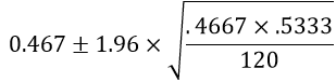
This calculation becomes 0.467 ± 0.089, which is the interval (0.378 → 0.556).  We can be 95% confident that between 37.8% and 55.6% of all students at the university would answer right front.  Notice that this interval lies completely above the value 0.25, consistent with our having rejected the null value of 0.25. 

Part (h) is an important question, as it prompts students to pause and consider that the sample of students in my class (or your class, if you try this activity) was not randomly selected from any population, so we should not take any of these inferences too seriously.  We should even be cautious about generalizing to all students at the university.  I recommend that students say that then results can be generalized only to a population of students similar to those in the sample.

---

I also use hypothetical data with the “which tire?” context to lead students to investigate the impact of sample size on hypothesis tests and confidence intervals.

5. Suppose that 30% of the people in a random sample from a population select the right front tire. 

• a) What more information do you need to conduct a hypothesis test and determine a confidence interval?
• b) Suppose that the sample size is n = 100.  Determine the value of the test statistic, p-value, and 95% confidence interval.
• c) Repeat for a sample size of n = 500.
• d) Summarize the role of sample size on these hypothesis tests and confidence intervals.  

Most students realize in part (a) that we need to know the sample size.  I encourage them to express this in context: We need to know how many people answered the “which tire” question.  I also encourage students to use technology (such as the applet here) for the calculations in parts (b) and (c), so they can focus on the underlying concept.

With a sample size of 100 in part (b), the z-test statistic is 1.15 with a p-value of 0.1241.  The sample result (30% saying “right front”) does not provide much evidence to conclude that right front would be selected more than by random chance.  The 95% confidence interval for the population proportion who would select the right front tire is (0.210 → 0.390), so we can be 95% confident that between 21.0% and 39.0% of all people would select the right front tire.  Notice that this interval includes the value 0.25.

With a sample size of 500 in part (c), the z-test statistic is 2.58 with a p-value of 0.0049.  The sample result (30% saying “right front”) provides strong evidence to conclude that right front would be selected more than by random chance.  The 95% confidence interval for the population proportion is (0.260 → 0.340), so we can be 95% confident that between 26.0% and 34.0% of all people would select the right front tire.  Notice that this interval is entirely above the value 0.25.

For part (d), I hope students say that when the sample result remains proportionally the same, a larger sample size produces a larger z-test statistic and smaller p-value.  This means that a larger sample size produces stronger evidence against the null hypothesis, in favor of the alternative that people tend to select the right front tire more often than would be expected by random chance.  A larger sample size also generates a more narrow confidence interval.

---

You have no doubt noticed that in the previous exercises, I converted the non-binary variable (which tire was picked) into a binary variable (right front or not).  The non-binary nature of the original variable provides a good opportunity for students to practice with applying chi-square goodness-of-fit tests.

6. Consider testing the null hypothesis that students are equally likely to select any of the four tires.  Here are the responses (counts) for my 120 students in the Winter quarter of 2017:

• a) Determine the expected counts for testing this hypothesis.
• b) Calculate the value of the test statistic.
• c) Determine the p-value.
• d) Summarize your conclusion.
• e) Identify the category (tire) with the largest contribution to test statistic, and comment on what the data reveal about this tire.
• f) Now test a new hypothesis: Students are twice as likely to select the right front tire as any other tire, and the rest are equally likely.  Report the hypothesis, test statistic, and p-value.  Summarize your conclusion.

The expected counts, under the null hypothesis of equal likeliness, are 120×(1/4) = 30 for each tire.  The chi-square test statistic turns out to be 0.533 + 5.633 + 22.533 + 2.700 = 31.4.  The p-value, based on 3 degrees of freedom, is 0.0000007.  With such a very small p-value, we conclude that the sample data provide overwhelming evidence to reject the hypothesis that students are equally likely to select among the four tire choices.  Not surprisingly, the largest contribution to the test statistic comes from the right front tire, where the observed count (56) considerably exceeds the expected count (30).  This reveals that the popularity of the right front tire is the biggest contributor to rejecting the null hypothesis of equal likeliness.

For part (f), students must first figure out that the proportions in the null hypothesis are now 0.4 for right front and 0.2 for each of the other tires.  Students then produce the following table as they conduct the test:

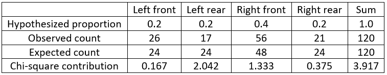
Now the p-value turns out to be 0.271, so the sample data do not provide convincing evidence to reject the 20-20-40-20 hypothesis.  Some students take this a step too far by concluding that the sample data provide evidence in favor of the 20-20-40-20 hypothesis*.  I like having students use a single dataset to test one hypothesis that produces a very small p-value and another that yields a not-so-small p-value. 

* See post #29 (Not enough evidence, here) for more examples and discussion about the perils of drawing conclusions when the p-value is not small.

---

This “which tire” question provides a fun context in which to gather data from students.  The data collection takes very little time.  You can then ask students to ponder several questions about the data that illustrate various aspects of statistical inference.

Before I close, I want to emphasize a concern that I mentioned, but only briefly, above: Needless to say, students in your class constitute only a convenience sample of students from your school.  You could make a strong case that performing statistical inference on such data is inappropriate.  I do think it’s important to draw students’ attention to this issue and caution them not to take their findings too seriously or generalize their results very broadly.  Nevertheless, I think this is a fun context that can be memorable for students, while allowing you to ask good questions about important topics in statistical inference.