#58 Lizards and ladybugs: illustrating the role of questioning

This guest post has been contributed by Christine Franklin. You can contact her at chris_franklin@icloud.com.
Chris Franklin has been one of the strongest advocates for statistics education at the K-12 level for the past 25 years. She has made a tremendous impact in this area through her writings and presentations, and also with her mentorship and leadership on individual levels. Her work includes the PreK-12 GAISE report (here), the Statistical Education of Teachers report (here), and a college-level textbook (here). Chris also served as Chief Reader of the AP Statistics program. Chris is retired from the Statistics Department at the University of Georgia, and she currently serves as the inaugural K-12 Statistical Ambassador for the American Statistical Association (read more about this here). I am very pleased that Chris agreed to write this guest blog post about the role of questioning described in the forthcoming revision of the PreK-12 GAISE report.
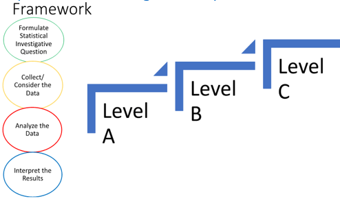
It has been my great fortune to be part of the writing teams for both the Pre-K-12 GAISE Framework published in 2005 (here) and the soon-to-be published Pre-K-12 GAISE II (tentatively planned for autumn release 2020)*. The GAISE Framework of essential concepts is built around the four-step statistical problem-solving process: formulate statistical investigative question, collect/consider data, analyze the data, and interpret the results. This framework involves three levels of statistical experience, with Level A roughly equivalent to elementary, B to middle, and C to high school. Question-posing throughout the statistical problem-solving process and at each of the progressive levels is essential:
* The GAISE II writing team, which also developed the examples presented in this post, includes Anna Bargagliotti (co-chair), Pip Arnold, Rob Gould, Sheri Johnson, Leticia Perez, and Denise Spangler.
This four-step statistical problem-solving process typically begins with formulating a statistical investigative question. When analyzing secondary data from an available source, the process might start with considering the data. The problem-solving process is not linear, and it is important to interrogate continuously throughout analyzing the data and interpreting the results. Posing good questions and knowing when to question is a skill that we must constantly hone. The GAISE II report presents 22 examples across the three levels to illustrate the necessity of being able to reason statistically and to make sense of data. Key within all these examples is the role of questioning. I will present two of my favorite examples from GAISE II to illustrate the crucial role of questioning.
Example 1: Those Adorable Ladybugs
1. Formulate Statistical Investigative Questions
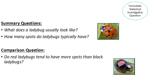
One of the new more science-focused investigations presented at Level A in GAISE II is about ladybugs. With beginning students, teachers might provide guidance when coming up with a statistical investigative question, the overarching question that begins the investigation. As students advance from Level A to Level B, students take more ownership in posing questions through the process. A statistical investigative question a student might pose is: What does a ladybug usually look like? or How many spots do ladybugs typically have? that ask for a summary. The statistical investigative question the student poses might also be comparative such as: Do red ladybugs tend to have more spots than black ladybugs? Questions for this step of the process are shown here:
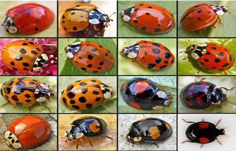
To answer these questions, we need to observe some ladybugs. Students might collect them outdoors. Teachers can also mail-order live ladybugs. An alternative is to use photo cards that allow students to observe a variety of ladybugs:
2. Collect/Consider Data – Data Collection Questions
To answer the statistical investigative questions posed by the students, data collection questions are developed. Some examples are given in the figure below:
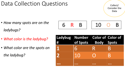
These questions collect data for one numerical variable (number of spots) and two categorical variables (color of body and color of spots). Collecting data requires careful measurement and even at this level, students will have to wrestle with questions such as: What is a spot versus a blemish? The class needs to agree upon some criteria as to what constitutes a spot. For example, they might decide not to count spots that are on the margins of the elytra, which is the hard wing cover.
How might young students organize the data? They could use data cards to organize the variable values for each ladybug, where each data card represents a case (the ladybug), as shown above. These physical data cards can assist beginning students to develop understanding on what is a ‘case’, a challenging concept for even advanced students. The students might next create a table, also as shown above.
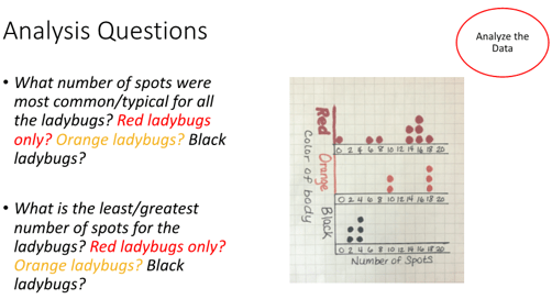
3. Analyze the Data – Analysis Questions
How do the students now make sense of the data? Beginning Level A students might use a picture graph that allows each ladybug to be identified. As students advance to Level B, they can use a dotplot. Teachers should support Level A students in thinking about the distribution and asking analysis questions. Analysis questions might prompt different representations or prompt the need for different data collection questions. This step is depicted here:
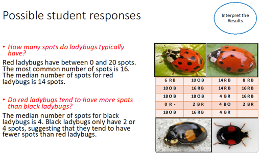
4. Interpret – Connecting to the Statistical Investigative Question
As the analysis questions are answered, the results of the data analysis aid in answering the statistical investigative question(s). Level A students are not expected to reason beyond the sample, and the teacher should encourage the students to state their conclusion in terms of the sample. Some possible student responses are shown here:
The ladybug investigation allows students at a young age to experience the statistical problem- solving process, recognize the necessity of always questioning throughout the process, and learn how to make sense of data by developing understanding of cases, variables, data types, and a distribution. These young students can also begin to experience that questioning through the statistical problem process is not necessarily linear – a typical upper-end Level B and Level C experience as illustrated with the following example.
Example 2: Those Cute Lizards
As students transition from Level B to Level C, they are becoming more advanced with the types of questions posed throughout the statistical problem-solving process, considering datasets that are larger and not necessarily clean for analysis, and using more tools and methods for analyzing the data.
1. Formulate Statistical Investigative Questions
Suppose students in a science class are investigating the impact of human development on wildlife. In an earlier analysis of a small pilot dataset, the students concluded that lizards in “disturbed” habitats (those with human development) tended to have greater mass than lizards in natural habitats. This led the students to pose and investigate the following question: Can a lizard’s mass be used to predict whether it came from a disturbed or a natural habitat?
2. Collect/Consider Data – Data Collection Questions
The students searched for available data that might help answer this statistical investigative question. They found a dataset where a biologist randomly captured individual lizards of one species across these two different habitats on four islands in the Bahamas (see research article here). The biologist found 81 lizards from natural habitats and 78 from disturbed habitats and recorded measurements on several different variables, as shown here:
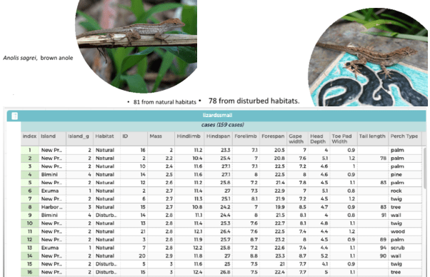
Students should explore and interrogate the dataset, asking what variables are included, what unit of measurement was used for each variable, and whether the variables will be useful and appropriate for answering the statistical investigative question. If the data are reasonable for investigating the posed statistical question, then the students will move to the analysis stage. If the data are not reasonable, they need to search for other data.
3. Analyze Data – Analysis Questions and Interpret
Recall the initial statistical investigative question: Can a lizard’s mass be used to predict whether it came from a disturbed or a natural habitat?
Students at Level B/C might first consider the distribution of mass for each of the two groups, asking appropriate analysis questions to compare the characteristics of those groups with respect to shape, center, variability, and possible unusual observations. The dotplots below, created in the Common Online Data Analysis Platform (CODAP, available here), display the distributions of mass (in grams) for the two types of lizards:
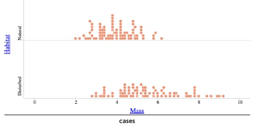
Students see considerable overlap in the two distributions but some separation. We want students to recognize that the more separation in the distributions, the better we can predict lizard habitat from mass. In thinking about how they can use these distributions to predict lizard habitat from mass, a student can consider a classification approach by asking: Where would you draw a cutoff line for the two distributions of mass to predict type of habitat?
Students might see a separation of the two distributions at around 6.25 grams, thus proposing the classification rule: If the lizard’s mass is less than 6.25 grams, then classify the lizard as from a natural habitat; otherwise, classify the lizard as from a disturbed habitat. Due to the significant overlap, many lizards would be mis-classified with this rule. Students can then count the number of mis-classifications with this rule, as shown here:
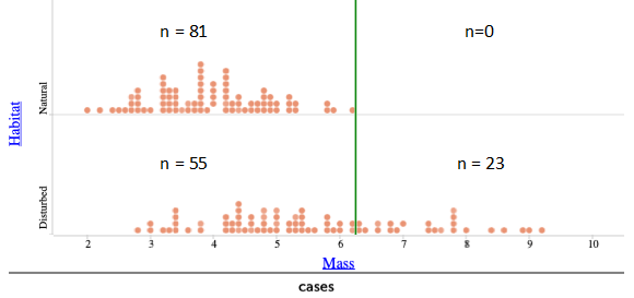
Students can then create a table/matrix and calculate the mis-classification rate to be 55/159 ≈ 0.346, or 34.6%:
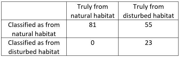
Should we be satisfied with a mis-classification rate of 35%, or can we improve with a different classification rule? We want students to revisit the two distributions of mass and consider finding a different cutoff point that will lower the mistakes made and reduce the mis-classification rate. Students may notice that if the cutoff point is lowered to 5 grams, we will mis-classify a few “natural” lizards but will correctly classify many more “disturbed” lizards:
The mis-classification rate becomes (32+11)/159 = 43/159 ≈ 0.270, or 27.0%, so this new classification rule reduces the mis-classification rate from 35% to 27%. Students can continue to develop other rules that further reduce the mis-classification rate.
Encourage students to be inventive as they develop more classification rules. They may soon be asking if there are others variables in the data set that may help in predicting the type of habitat in addition to mass. Thus, they now return to posing another possible statistical investigative question: Can a lizard’s mass and head depth be used to predict whether it came from a natural or disturbed habitat?
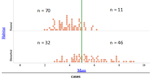
Now back at the analysis component of the statistical problem-solving process, a student at Level B/C may first explore the bivariate relationship between the two numerical variables, mass and head depth, by examining a scatterplot. Utilizing output from a web applet in ArtofStat (here), we notice a moderate positive linear relationship between mass and head depth. A line of best fit to the data yields the equation: predicted mass (grams) = -5.27 + 2.01×head depth (centimeters):
An analysis question at this stage could be: What is the interpretation of the slope 2.01? Since this is a probabilistic rather than deterministic model, we want students to say: For each one centimeter increase in head depth, the mass of the lizard is predictedto increase by 2.01 grams, on average.”
This analysis provides useful information, but it does not allow us to address our statistical investigative question to use mass and head depth to predict whether a randomly chosen lizard is from a natural or a disturbed habitat. How might we refine our analysis to incorporate type of habitat?
Instead of displaying the lizards in the scatterplot together ignoring their type of habitat, we can display the lizards using different symbols for natural and disturbed habitat. This provides a multivariate analysis where we have incorporated a third variable. The following graph displays the output from this analysis with separate lines of best fit for the two habitats:
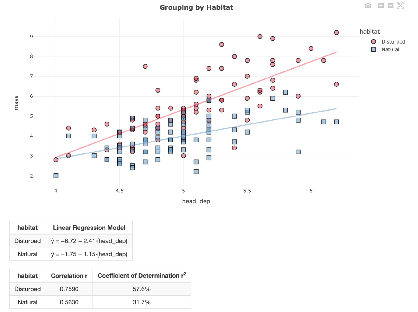
Now suppose a randomly chosen lizard has mass 3.6 grams and head depth 5.5 centimeters. Would you predict this lizard to be from a natural or disturbed habitat? How would you use the multivariate analysis to make this prediction?
Again, let students explore and try different approaches, asking students to justify their approach statistically. Some student approaches might be:
- A graphical approach: Plot the point (5.5, 3.6) on the scatterplot. This point lies closer to the prediction line for natural habitat than the prediction line for disturbed habitat. This point also falls more within the cluster of points for lizards from a natural than from a disturbed habitat.
- A computational approach: Evaluate the predicted mass based on a head depth of 5.5 cm for each of the two lines. The predictions turn out to be 5.05 grams for the “disturbed” line, 4.575 for the “natural” line. The residuals for these predictions are (3.6 – 5.05) = -1.45 for the “disturbed” group, (3.6 – 4.575) = -0.975 for the “natural” group. Because the residual for “natural” is closer to zero than the residual for “disturbed,” we predict that this lizard came from a natural habitat.
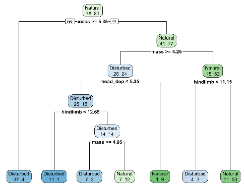
All of these analyzes will result in some mis-classifications. Our goal is to minimize the mis-classification rate. Looking back at the dataset of variables measured on the lizards by the biologists, students might consider if more variables could be included to improve classification accuracy. Again, students might return in the process to posing a new statistical investigation question: How can different features of a lizard (e.g., head depth, hind limb length, mass) be best used to predict whether it came from a natural or a disturbed habitat?
The analyses we have explored thus far can be generalized to more than two predictor variables, but developing classification rules becomes tedious without the use of computer technology. An algorithm known as Classification and Regression Tree (CART) produce a series of rules for making classifications based on a number of predictor variables. Below is a CART using mass, head depth, and hind limb length to predict type of habitat. The goal is that Level C students understand how to interpret output from the CART algorithm, not learn details of how the algorithm works.
Whether you are working with small samples from a population, experimental data, or vast datasets such as those found on public data repositories, questioning throughout the statistical problem-solving process is essential. This process typically starts with a statistical investigative question, followed by a study designed to collect data that aligns with answering the question. Analysis of the data is also guided by asking analysis questions. Constant interrogation of the data throughout the statistical problem-solving process can lead to the posing of new statistical investigative questions. When considering secondary data, the data first need to be interrogated.
The ladybug and lizard examples attempted to illustrate the essential role of questioning throughout the statistical process. Notice that the ladybug example involves summary and comparative investigative questions, while the investigative questions posed and explored in the lizard example are associative – looking for relationships among two or more variables to aid in making predictions.
Now more than ever, questioning is a vital part of being able to reason statistically. In carrying out the statistical problem-solving process, we want students and adults to always be asking good questions. The Pre-K-12 GAISE II documents advocates that this role of questioning begin at a very young age and gain maturity with age and experience.
To conclude with a quote from the GAISE II document: It is critical that statisticians, or anyone who uses data, be more than just data crunchers. They should be data problem solvers who interrogate the data and utilize questioning throughout the statistical problem-solving process to make decisions with confidence, understanding that the art of communication with data is essential.
P.S. A file containing the lizard data is available from the link here:
This guest post has been contributed by Christine Franklin. You can contact her at chris_franklin@icloud.com.

