#80 Power, part 1

I wish I had a better title for this post.  This one-word title reminds me of my two-part post about confounding variables, which I simply titled Confounding (see posts #43 and #44, here and here).  I tried to be clever with that title by arguing that the concept of confounding is one of the most confounding topics that students encounter in introductory statistics.  I suppose I could argue that the concept of power is one of the most powerful topics that students encounter, but my point is really that power is another topic that students find to be especially confounding.  I will abandon my search for cleverness and stick with this boring (but not misleading!) title.

I think we can help students to understand the concept of power by eliminating unnecessary terminology and calculations for our first pass at the topic.  We don’t need to mention null and alternative hypotheses, or rejection regions, or Type I and Type II errors, or p-values, or binomial or normal distributions, or expected value or standard deviation or z-score.  Don’t get me wrong: We’ll use most of those ideas, but we don’t need to let the terminology get in the way.

Instead we can present students with a scenario and an overarching question that you and I recognize as a question of power.  Then we can lead students to answer that big question by asking a series of smaller questions.  Questions that I pose to students appear in italics below.

---

Here’s the scenario that I use with my students: Suppose that Tamika is a basketball player whose probability of successfully making a free throw has been 0.6.  During one off-season, she works hard to improve her probability of success.  Of course, her coach wants to see evidence of her improvement, so he asks her to shoot some free throws. 

Here’s the overarching question: If Tamika really has improved, how likely is she to convince the coach that she has improved?  The other big question is: What factors affect how likely she is to convince the coach that she has improved?

I try not to over-do sports examples with my students, but I think the context here is very helpful and easy to follow, even for students who are not sports fans.

You won’t be surprised to see that we’ll use simulation as our tool to address these questions.

---

Let’s say that the coach gives Tamika 25 shots with which to demonstrate her improvement.

a) Suppose that she successfully makes 23 of the 25 shots.  Would you be reasonably convinced that she has improved?  Why or why not?

b) What if she makes 16 of the 25 shots – would you be reasonably convinced that she has improved?  Why or why not?

Most students realize that 60% of 25 is 15*, so both 16 and 23 are more successes that we would expect (for the long-run average) if she had not improved.  Their intuition suggests that 23 successes would provide very strong evidence of improvement, because it seems unlikely that a 60% shooter would achieve that many successes.  On the other hand, 16 successes does not provide strong evidence of improvement, because it seems that a 60% shooter could easily get a bit lucky and obtain 16 successes.

* You’re welcome to call this the expected value if you’d like.

c) What does your intuition suggest about how many shots Tamika would have to make successfully in order to be convincing? 

When I asked my students to type their answer to this question into the zoom chat during class a few days ago, nearly every student typed 20.  I said that this seemed reasonable and that we would proceed to use simulation to investigate this question a bit more carefully.  We used an applet (here) to conduct the simulation analysis.  The applet inputs required are:

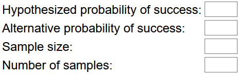
d) Which input values can you specify already?

The hypothesized probability of success is 0.6, and the sample size is 25.  Later we’ll assume that Tamika has improved to have a 70% chance of success, so we’ll enter 0.7 for the alternative probability of success.  I like to start with simulating just one sample at a time, so we’ll enter 1 for number of samples at first; later we’ll enter a large number such as 10,000 for the number of samples.

e) Click on “draw samples” five times, using 1 for the number of samples each time.  Did each of the simulated samples produce the same number of successful shots?

Part e) would be easy to skip, but I think it’s important.  This question forces students to acknowledge randomness, or sampling variability.  I don’t think any students struggle to answer this correctly, but I think it’s worth drawing their attention to this point.

f) Now enter 9995 for the number of samples, and click on “draw samples” to produce a total of 10,000 simulated sample results.  Describe the resulting distribution for the number of successes.  Comment on shape, center, and variability.

Here are some typical results:

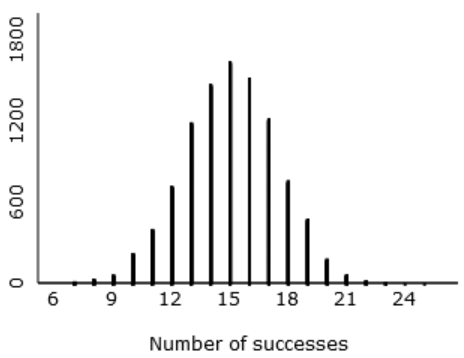
My students are quick to say that the shape of this distribution is symmetric, unimodal, normal-ish.  The center is near 15, which is what we expected because 60% of 25 is 15.  There’s a good bit of variability here: The simulated results show that Tamika sometimes made as few as 7 or 8 shots out of 25, and she also made as many as 23 or 24 shots out of 25.

g) Has this simulation analysis assumed that Tamika has improved, or that Tamika has not improved?

This is also a key question that is easy for students to miss: This simulation analysis has assumed that Tamika has not improved*.  We use the distribution of the number of successes, assuming that she has not improved, to decide how many successes she needs to provide convincing evidence of improvement.  I try to reinforce this point with the next question:

* You’re welcome to call this the null hypothesis.

h) Based on these simulation results, do you feel justified in your earlier answers about whether 23 successes, or 16 successes, would provide convincing evidence of improvement?  Explain.

Students who thought that 23 successes in 25 attempts provides very strong evidence of improvement should feel justified, because this simulation reveals that such an extreme result would happen only about 4 times in 10,000* (see graph on the left).  Similarly, students were correct to believe that 16 successes does not provide much evidence of improvement, because it’s not at all unlikely (better than a 40% chance*) for a 60% shooter to do that well (or better) by random chance (see graph on the right).

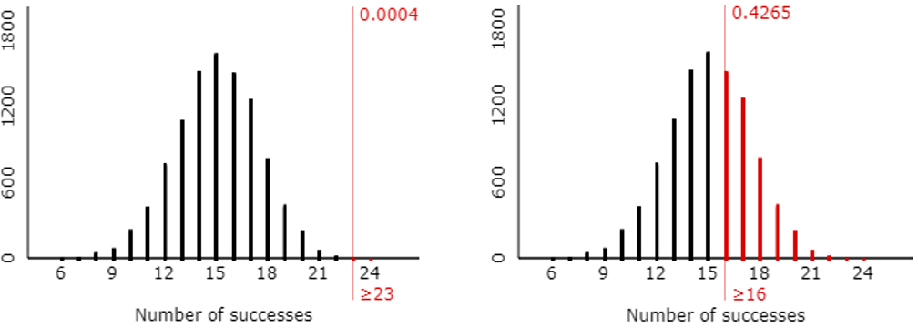
* You’re welcome to refer to these percentages as approximate p-values.  See post #12 (here) for an introduction to simulation-based inference.

---

Now we come to one of the harder questions:

i) Suppose that the coach decides on the following criterion for his decision rule: He’ll decide that Tamika has improved if her number of successes is large enough that such an extreme result would happen less than 5% of the time with a 60% shooter.  According to this rule, how many shots does Tamika need to make successfully to convince her coach?

I encourage students to answer this at first with trial-and-error.  Enter 17, and then 18, and so on into the “rejection region” box until you find the smallest number for which less than 5% of the simulated samples produce such a large number (or more) of successes.  The answer turns out to be that Tamika needs to make 20 or more of the 25 shots* to be convincing, as shown here:

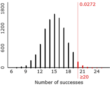
* You’re welcome to call this the rejection region of the test, especially as the applet uses that term.

I was quick to point out to my students how good their intuition was.  As I mentioned earlier, nearly all of my students who responded in the zoom chat predicted that Tamika would need to make 20 shots to be convincing.

Now, finally, we address the big picture question:

j) Make a guess for how likely Tamika is to make 20 or more shots successfully out of 25 attempts, if she has improved to a 0.7 probability of successfully making a single shot.

I don’t really care how well students guess here.  My point is to remind them of the big question, the reason we’re going through all of this.  Next we use the applet to conduct another simulation to answer this question:

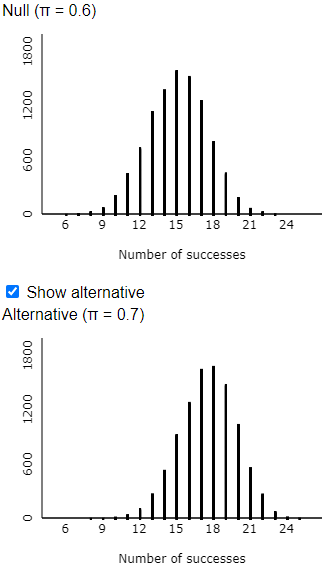
k) Check the “show alternative” box in the applet, which displays the distribution of number of successes, assuming that Tamika has improved to a 0.7 probability of success.  Do you see much overlap in the two distributions?  Is this good news or bad news for Tamika?  Explain.

There is considerable overlap in the two distributions, as shown here:

l) According to the applet’s simulation results, in what percentage of the 10,000 simulated samples does Tamika, with a 70% chance of making a single shot, do well enough to convince the coach of her improvement by successfully making 20 or more shots?  Would you say that Tamika has a good chance of demonstrating her improvement in this case?

Unfortunately for Tamika, she does not have a good chance of demonstrating her improvement.  In my simulation result shown here, she only does so about 19.5% of the time:

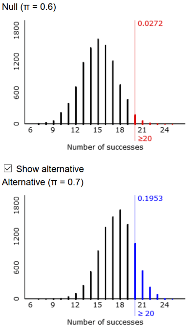
Here’s where we introduce the term of the day: We have approximated the power of this test.  Power in this case represents the probability that Tamika convinces her coach that she has improved, when she truly has improved.

---

Now we’ll begin to consider factors that affect power, first by asking:

m) What would you encourage Tamika to request, in order to have a better chance of convincing the coach that she has improved?

Several of my students responded very quickly in the zoom chat to say: more shots*.

* You’re welcome to call this a larger sample size.

n) Now suppose that the coach offers 100 shots for Tamika to show her improvement.  Re-run the simulation analysis.  Is there more, less, or the same amount of overlap in the two distributions?  Is this good news or bad news for Tamika?  Explain.

The simulation results reveal that the larger sample size leads to much less overlap between these two distributions:

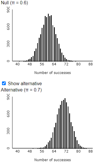
This is very good news for Tamika, because this shows that it’s easier to distinguish a 70% shooter from a 60% shooter when she takes 100 shots than with only 25 shots.

o) How many shots must she now make successfully in order to convince the coach?  How does this compare to the percentage of 25 shots that she needs to make in order to be convincing?

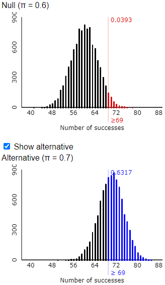
The following graph shows that making 69 or more shots is sufficient to convince the coach that she has improved from a 60% shooter:

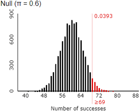
Recall that with 25 shots, Tamika had to make 20 of them to be convincing, so the percentage that she needs to make has decreased from 80% to 69% with the increase in sample size.

p) What is the (approximate) probability that Tamika will be able to convince the coach of her improvement, based on a sample of 100 shots?  How has this changed from the earlier case in which she could only take 25 shots?

This output shows that she has about a 63% chance of convincing the coach now:

This probability is more than three times larger than the previous case with only 25 shots.

q) What else could Tamika ask the coach to change about his decision process, in order to have a better chance to convince him of her improvement?

This one is much harder for students to suggest than sample size, but someone eventually proposes to change the 5% cut-off value, the significance level.  Making that larger would mean that the coach is requiring less strong evidence to be convincing, so that will increase Tamika’s chances of convincing the coach.

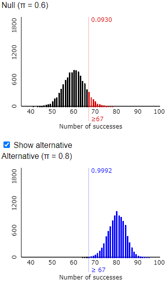
r) Change the coach’s significance level from 0.05 to 0.10.  How does this change the number of shots that Tamika must make to convince the coach of her improvement?  How does this change the probability that she convinces the coach of her improvement?

As shown in the following output, Tamika now only needs to make 67 shots, rather than 69, in order to convince the coach.  The probability that she achieves this as a 70% shooter is approximately 0.777, which is considerably larger than the previous probability of approximately 0.632.

s) Identify one more factor that affects how likely Tamika is to convince the coach that she has improved.

I sometimes give a hint by suggesting that students think about the applet’s input values. Then someone will suggest that Tamika could try to improve more.

t) Now suppose that Tamika improves so much that she has a 0.8 probability of successfully making a single shot.  How does this change the number of shots that Tamika must make to convince the coach of her improvement?  How does this change the probability that she convinces the coach of her improvement?

I tell students that they do not need to use the applet to answer the first of these questions.  This change does not affect how many shots she must make to convince the coach.  That value depends only on her previous probability of success, not her new and improved probability of success.  But her new success probability will produce even greater separation between the two distributions and will increase her probability of convincing the coach.  The following output reveals that the new probability is approximately 0.999:

---

This activity can introduce students to the concept of power without burdening them with too much terminology or too many calculations.  I grant that it’s very convenient to use terms such as significance level and rejection region and power, but I prefer to introduce those after students have first explored the basic ideas.

In the second post in this series, I will discuss some common questions from students, describe some assessment questions that I used for this topic, including some that I now regret, and present extensions of this activity for introducing the concept of power to more mathematically inclined students.