#85 Three assignments in one
I give a lot of quizzes in my classes. I have been giving even more than usual this year while teaching remotely, and I’ve revised them to an auto-graded format. I’ve written about such quizzes in many posts*.
* My most recent post of this type was #83, titled Better, not necessarily good, here.
I also give longer assignments that ask students to analyze data and submit a report that answers a series of questions. This post discusses my most recent assignment of this type.
At the risk of prompting you to stop reading now, I confess that the questions in this assignment are quite straight-forward. I think this assignment is worthwhile for my students, because it asks them to use JMP software to analyze raw data for themselves, as compared to quizzes and exams on which I provide students with output and summaries.
Although there’s nothing particularly original or clever about this assignment, I do like two aspects. One is that it covers several topics with one dataset. Students apply a chi-square test, analysis of variance, and a test about correlation on different pairs of variables. They also produce appropriate graphs and summary statistics prior to conducting those tests. Students need to select the correct procedure to address a particular question, although JMP software provides a big assist with that.
I also like that the results of two of the three tests do not come close to achieving statistical significance. I sometimes worry that I present too many examples with very small p-values, so this assignment can remind students that not all studies discover significant differences among groups.
As always, questions that I pose to students appear in italics.
Here’s background information about the study that I provided to students:
An article* reported on a study in which 160 volunteers were randomly assigned to one of four popular diet plans: Atkins, Ornish, Weight Watchers, and Zone (40 subjects per diet). These subjects were recruited through newspaper and television advertisements in the greater Boston area; all were overweight or obese with body mass index values between 27 and 42. Among the variables recorded were:
- which diet the subject was assigned to
- whether or not the subject completed the twelve-month study
- the subject’s initial weight (in kilograms)
- the degree to which the subject adhered to the assigned diet, taken as the average of 12 monthly ratings, each on a 1-10 scale (with 1 indicating complete non-adherence and 10 indicating full adherence)
- the subject’s weight after 12 months (in kilograms)
- the subject’s weight loss after twelve months (in kilograms, with a negative value indicating weight gain)
* You can find the JAMA article about this study here. A link to the dataset appears at the end of this post.
- a) For each of the six variables (in the bullet points above), indicate whether the variable is categorical (also binary?) or numerical.
My students are used to this question, as are regular readers of this blog*. I’m trying to set students up in good position to decide which technique to apply for each of the three sets of questions to come. Frankly, I doubt that many students think that through. When they ask questions in office hours about how to proceed with a given question, they often seem to be surprised when I point out that earlier questions in an assignment often prepare them to answer later questions.
* See post #11, titled Repeat after me, here, in which I argue for asking these questions at the beginning of (almost) every example in the course.
The first two variables listed here are categorical, with the second one binary and the first one not. The other four variables are numerical.
I probably should have asked two additional questions, with which my students are also very familiar, at this point: Was this an observational study or an experiment? Did this study make use of random sampling, random assignment, both, or neither? I decided not to ask these questions in this assignment only because it grew to be quite long.
First we will investigate whether the sample data provide strong evidence that different diets produce different amounts of weight loss, on average.
- b) Use JMP to produce dotplots and boxplots of the distributions of weight loss for the four diet groups.
- c) Use JMP to calculate means and standard deviations of weight loss for the four diet groups.
- d) Do the technical conditions for the ANOVA F-test appear to be satisfied? Explain.
- e) Use JMP to produce the ANOVA table.
- f) Report the null hypothesis being tested, using appropriate symbols. Report the value of the F-test statistic and p-value. Would you reject the null hypothesis at the α = 0.10 significance level? Summarize your conclusion from the ANOVA F-test.
This is the first course in which I have used JMP, which I am learning for the first time myself. I provided my students with a data file and fairly detailed instructions about how to use JMP to generate the requested output. Here are the graphs and summary statistics:
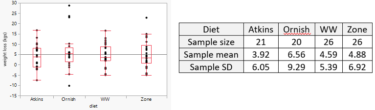
For the technical conditions of the ANOVA F-test, I want students to check three things: 1) This experiment made use of random assignment. 2) The dotplots and boxplots do not suggest strong skewness or outliers, so assuming that the weight loss amounts follow normal distributions is reasonable. 3) The ratio of the largest group SD to the smallest group SD is 9.29/5.39 ≈ 1.72 is less than 2, so it’s reasonable to assume that the standard deviations of weight loss among the groups are the same.
JMP produces the following ANOVA table:
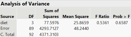
The null hypothesis to be tested is that all four diets have the same population mean weight loss: μA = μO = μW = μZ. The value of the test statistic is F = 0.5361, and the p-value is 0.6587. This p-value is not small in the least, so the sample data are not at all inconsistent with the null hypothesis that the four diets have the same population mean weight loss. We would not reject the null hypothesis at the α = 0.10 level, or at any other reasonable significance level. The sample data from this experiment provide no evidence that the four diets differ with regard to population mean weight loss.
Next we will investigate whether subjects were more or less likely to complete the study depending on which diet they had been assigned.
- g) Identify the name of the appropriate test to investigate this question.
- h) Use JMP to produce an appropriate graph and table to investigate this question.
- i) Which diet group(s) had the largest percentage of subjects who completed the study? What was the value for that percentage?
- j) Report the null hypothesis being tested. Also report the value of the test statistic and p-value. Would you reject the null hypothesis at the α = 0.10 significance level? Summarize your conclusion from this test.
I received more questions in office hours about part (g) than about any other part. I always responded by asking about the types of variables involved. When students told me that both variables are categorical, and only one variable is binary, I asked what test is appropriate for such data. For the students who answered that they did not know, I directed them to the appropriate section of their notes. The answer I’m looking for is a chi-square test for comparing proportions between multiple groups*.
* I really dislike the phrase “homogeneity of proportions.” I don’t see the value of asking students to use a six-syllable word that they might not even understand the meaning of. I like “chi-square test of homogeneity” even less, because that leaves open the question: homogeneity of what?
Here are a graph and table of counts:

Once again I think it’s a bit unfortunate that JMP automatically selects an appropriate graph after the user indicates the two variables of interest. The answer to (i) is that the Weight Watchers and Zone diets both had the largest completion percentages: 26/40 = 0.65, so 65% of those assigned to one of these diets completed the study.
JMP produces the following output for the chi-square test:

The usual chi-square statistic is the Pearson value 3.158, with a p-value of 0.3678. Once again the sample data do not provide evidence to conclude that the four diets differ, this time with regard to likelihood of completion.
Finally, we will investigate whether the data reveal a significant positive association between degree of adherence to the diet and weight loss.
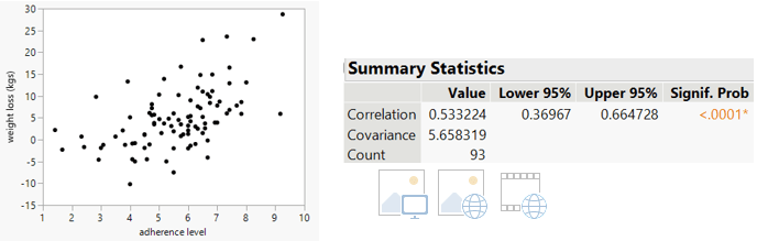
- k) Use JMP to produce an appropriate graph to investigate this question.
- l) Use JMP to calculate the value of the correlation coefficient between these variables.
- m) Calculate the value of the appropriate t-test statistic by hand. Also report the p-value from the JMP output. Summarize your conclusion.
Here’s a scatterplot of weight loss vs. adherence score, with a correlation coefficient of r = 0.533:
Calculating the value of this t-statistic is the only test statistic calculation that students complete by hand in this assignment. I could have asked them to produce regression output with this test statistic, but we had not yet studied regression when I gave this assignment. The calculation is:
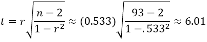
This test statistic reveals that the sample correlation coefficient of 0.533 is about six standard errors away from zero, so the p-value is extremely small, very close to zero. (The very small p-value can also be seen in the output above.) The sample data provide very strong evidence that weight loss is positively associated with adherence level in the population of all overweight people looking to lose weight with a popular diet.
Several students asked in office hours about the sample size to use in this calculation. They noted that the overall sample size for the chi-square test was 160, but they realized that using 160 for n in the correlation test statistic calculation did not seem right. I simply asked how many people have values of weight loss and adherence level that went into calculating the correlation coefficient. Students quickly realized that this calculation restricts attention to the 93 subjects who completed the study.
In case you might be wondering about how this assignment is graded, I will now show the grading guidelines that I provided to my grader*. I encouraged my students to work in groups of 2-3 students on this assignment, but many students opted to work alone. This assignment generated 75 submissions among my 131 students, so there’s a lot of grading to be done. I tried to make the guidelines clear and specific, but I also tried to avoid making them so detailed that they would take a lot of time to apply.
* My grader Melissa in a third-year business major who is minoring in statistics. She has been extremely helpful to me, including catching an error in my solution to this assignment as she started her grading.
Here are my grading guidelines, for a total of 20 points:
- a) 1.5 pts. Take -.5 if 1-2 of the 6 answers are incorrect. Take -1 if 3-5 of the 6 answers are incorrect.
- b) 1 pt. Give .5 pt for the dotplots, .5 pt for the boxplots. It’s ok if the graphs are horizontal rather than vertical. Take -1 if the graphs are not separated by diet.
- c) 1 pt. Take -.5 if any values are missing or incorrect. Do not bother to check their values closely.
- d) 2 pts. Give .5 pt for overall answer of yes. Give.5 pt for mentioning random assignment (if they say random sampling but not random assignment, take -.5). Give .5 pt for mentioning normality; it’s fine if they say that the data do not look close enough to normal. Give .5 pt for comparing rato of largest/smallest SD to 2; if they just say “SD condition ok” without checking this ratio, take -.5.
- e) 1 pt.
- f) 2.5 pts. Give .5 pt for null (either symbols or words are ok, don’t need both), .5 pt for F and p, .5 pt for “do not reject null,” 1 pt for conclusion in context
- g) 1 pt. It’s ok to say just “chi-square test” or “chi-square test of independence” or “chi-square test of equal proportions.” Take -.5 pt for saying “chi-square test of goodness-of-fit.” Take -1 for not mentioning “chi-square” at all.
- h) 2 pts. Give 1 pt for graph, 1 pt for table. Take -.5 pt if variables are switched in graph.
- i) 1 pt. Give .5 pt for identifying WW and Zone as the two diets. Give .5 pt for correct proportion or percentage.
- j) 2.5 pts. Give .5 pt for null (either symbols or words are ok, don’t need both), .5 pt for X2 and p (it’s ok if these are off a bit due to rounding), .5 pt for “do not reject null,” 1 pt for conclusion in context
- k) 1 pt.
- l) 1 pt. It’s ok to have some rounding discrepancy.
- m) 2.5 pts. Give 1 pt for test stat (take -.5 for right idea but a mistake somewhere, such as using the wrong sample size), .5 pt for p-value (ok to say approx. zero), 1 pt for conclusion in context
P.S. The data file can be downloaded from the link below:


Trackbacks & Pingbacks