#34 Reveal human progress, part 2
In the previous post (here), I put my Ask good questions mantra on a temporary hold as I argued for another three-word exhortation that I hope will catch on with statistics teachers: Reveal human progress. In this post I will merge these two themes by presenting questions for classroom use about data that reveal human progress.
The first three of these questions present data that reveal changes over time. I think these questions are appropriate not only for introductory statistics but also for courses in quantitative reasoning and perhaps other mathematics courses. The fourth question concerns probability, and the last two involve statistical inference.
As always, questions that I pose to my students appear in italics.
1. The following graph displays how life expectancy has changed in South Africa over the past few decades:
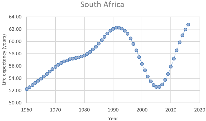
- a) Describe how life expectancy has changed in South Africa over these years.
- b) In which of these three time periods did life expectancy change most quickly, and in which did it change most slowly: 1960 – 1990, 1990 – 2005, 2005 – 2016?
- c) Explain what happened in South Africa in 1990 – 2005 that undid so much progress, and also explain what happened around 2005 to restart the positive trend. (You need to use knowledge beyond what’s shown in the graph to answer this. Feel free to use the internet.)
Question (a) is meant to be straightforward. I expect students to comment on the gradual increase in life expectancy from 1960 – 1990, the sudden reversal into a dramatic decline from 1990 – 2005, and then another reversal with an even more rapid increase from 2005 – 2016. A more thorough response would note that the life expectancy in 2005 had plunged to a level about equal to that of 1965, and the life expectancy in 2016 had rebounded to exceed the previous high in 2005.
Question (b) addresses rates of change. I have in mind that students simply approximate these values from the graph. Life expectancy increased from about 52 to 62 years between 1960 and 1990, which is an increase of about 10 life expectancy years over a 30-year time period, which is a rate of about 0.33 life expectancy years per year*. From 1990 – 2005, life expectancy decreased by almost 10 years, for a rate of about 0.67 life expectancy years per year. The years between 2005 – 2016 saw an increase in life expectancy of about 10 years, which is a rate of about 1 life expectancy year per year. So, the quickest rate of change occurred in the most recent time period 2005 – 2016, and the slowest rate of change occurred in the most distant time period: 1960 – 1990.
* Unfortunately, the units here (life expectancy years per year of time) are tricky for students to express clearly. This can be one of the downsides of using real data in an interesting context.
It usually takes students a little while to think of the explanation in part (c), but some students eventually suggest the HIV/AIDS epidemic that devastated South Africa in the 1990s. Fortunately, effective medication became more available, helping to produce the dramatic improvement that began around the year 2005.
2. The following graph adds to the previous one by including the life expectancy for Ghana, as well as South Africa, over these years:
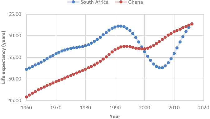
- a) Compare and contrast how life expectancy changed in these two countries over these years.
- b) Which country had a larger percentage increase in life expectancy over these years? Explain your answer without performing any calculations.
- c) Suppose that you were to calculate the changes in life expectancy for each year by subtracting the previous year’s value. Which country would have a larger mean of its yearly changes? Which country would have a larger standard deviation of its yearly changes? Explain your answers.
For part (a), I expect students to respond that Ghana did not experience the dramatic reversals that South Africa did. More specifically, Ghana experienced only a slight decline from about 1995 – 2000, much less dramatic and briefer than South Africa’s precipitous drop from 1990 – 2005. For full credit I also look for students to mention at least one other aspect, such as:
- Ghana had a much lower life expectancy than South Africa in 1960 and had a very similar life expectancy in 2016.
- Ghana’s increase in life expectancy since 2005 has been much more gradual than South Africa’s steep increase over this period.
The key to answering part (b) correctly is to realize that the two countries ended with approximately the same life expectancy, but Ghana began with a much smaller life expectancy, so the percentage increase is larger for Ghana than for South Africa.
Part (c) is not at all routine, requiring a lot of thought. Because Ghana had a larger increase in life expectancy over this time period, Ghana would have a larger mean for the distribution of its yearly changes. But South Africa had steeper increases and decreases than Ghana, so South Africa would have more variability (and therefore a larger standard deviation) in its distribution of yearly changes*.
* The means of the yearly changes turn out to be 0.302 years for Ghana, 0.188 years for South Africa. The standard deviations of the yearly changes are 0.625 years for South Africa, 0.174 years for Ghana.
3. Consider the following graph of energy-related carbon dioxide (CO2) emissions (in million metric tons) in the United States from 1990 – 2005:
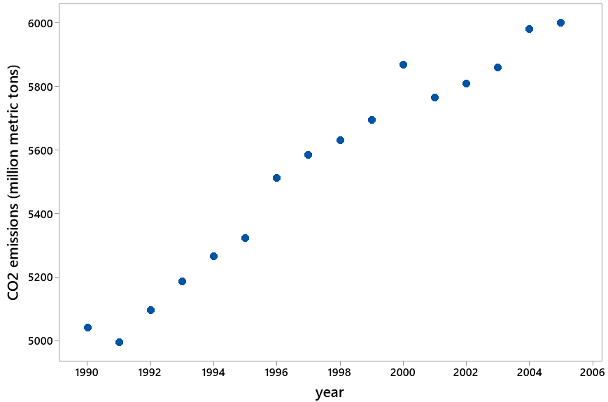
- a) Describe what the graph reveals.
- b) Determine the least-squares line for predicting CO2 emissions from year.
- c) Interpret the value of the slope coefficient.
- d) Use the line to predict CO2 emissions for the year 2018.
- e) The actual value for CO2 emissions in 2018 was 5269 million metric tons. Calculate the percentage error of the prediction from the actual value.
- f) Explain what went wrong, why the prediction did so poorly.
Students have little difficulty with part (a), as they note that CO2 emissions are increasing at a fairly steady rate from about 5000 million metric tons in 1990 to about 6000 million metric tons in 2005. I intend for students to use technology to determine the least squares line in (b), the equation of which turns out to be: predicted CO2 emissions = -135,512 + 70.61 × year.
To interpret the slope coefficient in part (c), students should respond that the predicted CO2 emissions increases by 70.61 million metric tons for each additional year. Using this line to predict CO2 emissions for the year 2018 in part (d) gives: -135,512 + 70.61 × 2018 ≈ 6979 million metric tons.
This prediction is not very close to the actual value of CO2 emissions in 2018, as it over-predicts by more than 1700 million metric tons. The percentage error for part (e) is: (6979 – 5269) / 5269 × 100% ≈ 32.5%.
The explanation in part (f) is that we should have been cautious about extrapolation. By using the least squares line to make a prediction thirteen years into the future, we assumed that the linear increasing trend would continue in the years following 2005. We did not have a good justification for making this assumption.
In fact, a graph of the entire dataset from 1990 – 2018 reveals that the increasing trend from 1990 – 2005 actually reversed into a decreasing trend from 2005 – 2018:
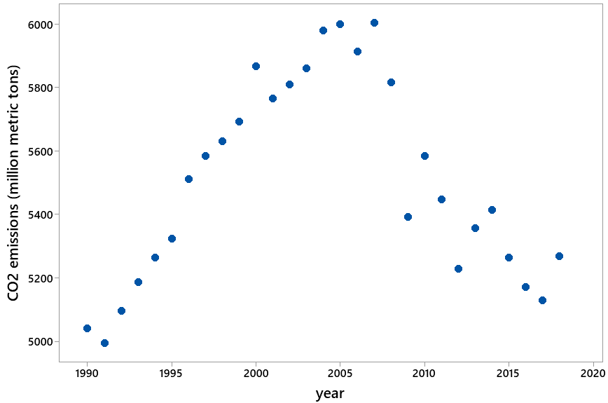
Students find these data to be very surprising. I hope the surprise aspect helps to make the caution about extrapolation memorable for them.
The next three questions concern Hans Rosling’s Gapminder/Ignorance Test. I presented three of the twelve questions on this test in the previous post (here). Each of the twelve questions asks respondents to select one of three options. The correct answer for each question is the most optimistic of the three options presented.
4. Suppose that all people select randomly among the three options on all twelve questions. Let the random variable X represent the number of questions that a person would answer correctly.
- a) Describe the probability distribution of X. Include the parameter values as well as the name of the distribution.
- b) Determine and interpret the expected value of X.
- c) Determine the probability that a person would obtain exactly the expected value for the number of correct answers.
- d) Determine and compare the probabilities of correctly answering fewer than the expected value vs. more than the expected value.
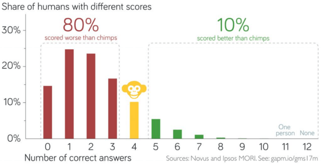
- e) Discuss how the actual survey results, as shown in the following graph, compare to the binomial distribution calculations.
Under the assumption of random selection among the three options on all twelve questions, the probability distribution of X, the number of correct answers, would follow a binomial distribution with parameters n = 12 and p = 1/3. A graph of this probability distribution is shown here:
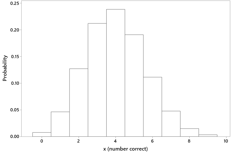
The expected value of X can be calculated as: E(X) = np = 12×(1/3) = 4.0. This means that if the questions were asked of a very large number of people, all of whom selected randomly among the three options on all twelve questions, then the average number of correct answers would be very close to 4.0.
The binomial probabilities in (c) and (d) can be calculated to be 0.2384 for obtaining exactly 4 correct answers, 0.3931 for 4 or fewer correct, and 0.3685 for more than 4 correct.
The survey data reveal that people do much worse on these questions that they would with truly random selections. For example, about 80% of respondents got fewer than four correct answers, whereas random selections would produce about 39.31% with fewer than four correct answers. On the other side, about 10% of people answered more than four questions correctly, compared with 36.85% that would be expected from random selections.
5. When the question about how the proportion of the world’s population living in extreme poverty has changed over the past twenty years, only 5% of a sample of 1005 respondents in the United States gave the correct answer (cut in half), while 59% responded with the option furthest from the truth (doubled).
- a) Determine the z-score for testing whether the sample data provide strong evidence that less than one-third of all Americans would answer correctly.
- b) Summarize your conclusion from this z-score, and explain the reasoning process behind your conclusion.
- c) Determine a 95% confidence interval for the population proportion who would answer that the rate has doubled.
- d) Interpret this confidence interval.
The z-score in (a) is calculated as: z = (0.05 – 1/3) / sqrt[(1/3)×(2/3)/1005] ≈ -19.1. This is an enormous z-score, indicating that the sample proportion who gave the correct response is more than 19 standard deviations less than the value one-third. Such an extreme result would essentially never happen by random chance, so the sample data provide overwhelming evidence that less than one-third of all adult Americans would have answered correctly.
The 95% confidence interval for the population proportion in part (c) is: .59 ± 1.96 × sqrt(.59×.41/1005), which is .59 ± .030, which is the interval (.560 → .620). We can be 95% confident that if this question were asked of all adult Americans, the proportion who would give the most wrong answer (doubled) would be between .560 and .620. In other words, we can be 95% confident that between 56% and 62% of all adult Americans would give the most wrong answer to this question.
I asked my students the question about how the extreme poverty rate has changed, before revealing the answer. The table below shows the observed counts for the three response options in a recent class:

6. Conduct a hypothesis test of whether the sample data provide strong evidence against the hypothesis that the population of students at our school would be equally likely to choose among the three response options.
The null hypothesis is that students in the population would be equally likely to select among the three options (i.e., that one-third of the population would respond with each of the three options). The expected counts (under this null hypothesis) are 83/3 ≈ 27.667 for each of the three categories. All of these expected counts are larger than five, so a chi-square goodness-of-fit test is appropriate. The chi-square test statistic turns out to equal 7.253, as shown in the following table:

The p-value, from a chi-square distribution with 2 degrees of freedom, is ≈ 0.027. This p-value is fairly small (less than .05) but not very small (larger than .01), so we can conclude that the sample data provide fairly strong evidence against the hypothesis that students in the population would be equally likely to select among the three options. The sample data suggest that students are more likely to give the most pessimistic answer (doubled) and less likely to give the most optimistic, correct answer (cut in half). This conclusion should be regarded with caution, though, because the sample (students in my class) was not randomly selected from the population of all students at our school.
The six questions that I have presented here only hint at the possibilities of asking questions that help students to learn important statistical content while also exposing them to data that reveal human progress. I also encourage teachers to point their students toward resources that empower them to ask their own questions, and analyze data of their own choosing, about the state of the world. I listed several websites with such data at the very end of the previous post (here).
P.S. The life expectancies for South Africa and Ghana were obtained from the World Bank’s World Development Indicators dataset, accessed through google (here). Life expectancy is defined here as “the average number of years a newborn is expected to live with current mortality patterns remaining the same.” The data on CO2 emissions were obtained from the United States Energy Information Administration (here). The data on the Gapminder/Ignorance Test were obtained from a link here.
Files containing the data on life expectancies and CO2 emissions can be downloaded from the links below:

Trackbacks & Pingbacks