#35 Statistics of illumination, part 4
In previous posts (here, here, and here), I described examples that I present on the first day of a statistical literacy course and also when I give talks for high school students. These activities show how data analysis can shed light on important questions and illustrate statistical thinking.
This post returns to this theme and completes the series. Today’s example highlights multivariable thinking, much like post #3 (here) that introduced Simpson’s paradox. One difference is that today’s example includes two numerical variables rather than all categorical ones. A similarity is that we begin with a surprising finding about two variables that makes perfect sense after we consider a third variable.
As always, questions that I pose to students appear in italics.
We will examine data on lung capacity, as measured by a quantity called forced expiratory volume (to be abbreviated FEV), the amount of air an individual can exhale in the first second of forceful breath (in liters). The following graph displays the distributions of FEV values for 654 people who participated in a research study, comparing smokers and non-smokers:

Which group – smokers or non-smokers – tends to have larger lung capacities? Does this surprise you? Students are quick to point out that although the two groups’ FEV values overlap considerably, smokers generally have higher FEV values, and therefore greater lung capacities, than non-smokers. Next I tell students that the average FEV values for the two groups are 2.57 liters and 3.28 liters. Which average is for smokers and which for non-smokers? Students realize from the graph that the larger average FEV belongs to the smokers.
Then I show boxplots of the distributions of FEV values. Without going into any of the calculation details, I simply explain that the boxplots present the 25th, 50th, and 75th percentiles of the distributions, along with the minimum and maximum, with outliers shown as asterisks:
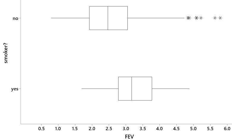
Describe how the distributions of FEV values compare between smokers and non-smokers. The key point here is that smokers have higher FEV values than non-smokers throughout the distributions (at the minimum, 25th and 50th and 75th percentiles), except near the maximum values. Non-smokers also have more variability in FEV values, including several outliers on the large side.
Does every smoker have a larger FEV value than every non-smoker? No, many non-smokers have a larger FEV value than many smokers. In others words, the FEV values overlap considerably between the two groups. What is meant by a statistical tendency in this context? This question is difficult but crucial to statistical thinking. I don’t make a big deal of this on the first day of class, but I point out that a statistical tendency is not a hard-and-fast rule. I emphasize phrases like on average and tend to and generally, in the hope that students will begin to catch on to probabilistic rather than deterministic thinking*.
* I am reminded of a book called How to Think Straight About Psychology, by Keith Stanovich, which includes a chapter titled “The Achilles Heel of Human Cognition: Probabilistic Reasoning.”
At this point I want students to focus on the big question: What in the world is going on here?? Why do smokers tend to have larger lung capacities than non-smokers?
I have withheld a very important piece of information until now: These 654 people were all children! Their ages varied from 3 to 19 years old, as shown in the following histogram:
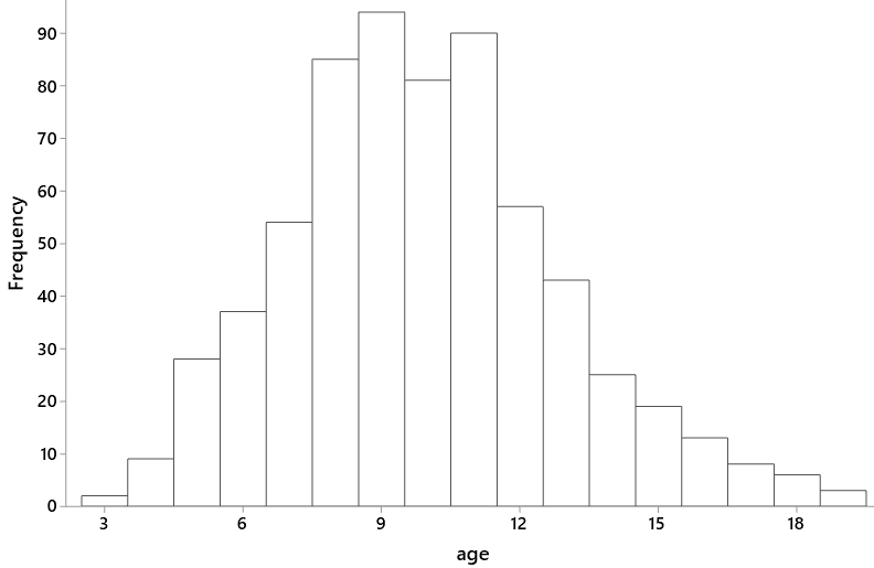
Before we analyze the data further, I ask students to think about this question in the back of their minds: How might this revelation about ages explain the surprising finding that smokers tend to have larger lung capacities than non-smokers?
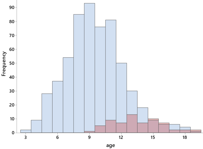
Now, for the front of students’ minds, I ask: How do you expect the distribution of age to differ between smokers and non-smokers? They naturally expect the smokers to be older children, while non-smokers include all of the younger and some of the older children. This prediction is confirmed by this graph:
Then we consider the remaining pair of variables that we have not yet analyzed: What do you expect to see in a graph of lung capacity (FEV) vs. age? Most students anticipate that lung capacity tends to increase as age increases. This is confirmed by the following graph:
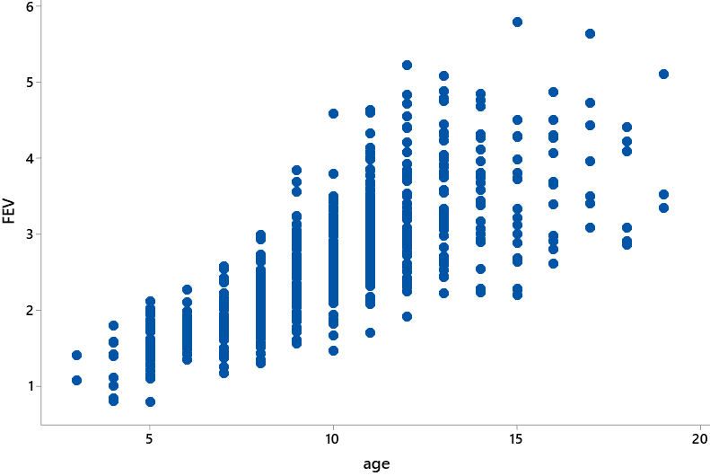
Do these last two graphs reveal a statistical tendency rather than a hard-and-fast rule? Yes, absolutely. Smokers tend to be older than non-smokers, but some smokers are younger than some non-smokers. Furthermore, older children tend to have greater lung capacities than younger children, but the scatterplot also reveals that some older children have smaller lung capacities than younger ones.
Now let’s analyze a graph that displays all three of these variables simultaneously. But first I ask students to take a step back and make sure that we’re all on the same page: What are the observational units, and what are the three variables here? Also classify each variable as categorical or numerical. The observational units are the 654 children. The three variables are age (numerical), lung capacity as measured by FEV (numerical), and whether or not the person is a smoker (categorical).
How can we include all three variables in one graph? This is a harder question, but some students astutely suggest that we can code the dots in the scatterplot of FEV vs. age with different colors or symbols to indicate smoking status.
Here’s the coded scatterplot, with blue circles for non-smokers and red squares for smokers:
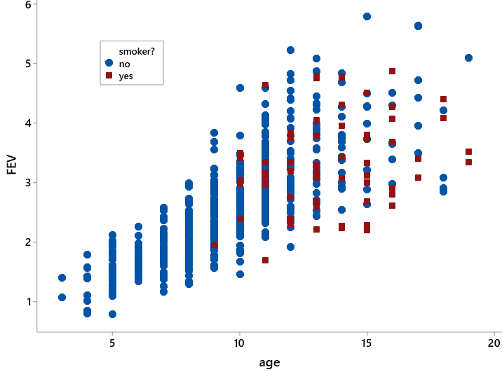
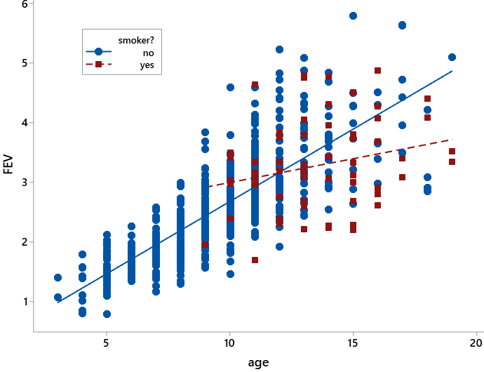
This graph contains a lot of noise, so it’s hard to discern much. We can see the overall patterns much more clearly by including lines of best fit* for the two groups:
* I’m not a fan of this phrase, but I don’t want to introduce least squares on the first day of class.
What does this graph reveal about lung capacities of smokers and non-smokers? I am hoping for two particular responses to this question, so after some initial discussion I often need to ask more pointed questions, starting with: For those older than age 12, which line predicts greater lung capacity: smokers or non-smokers? Does this surprise you? Students realize, of course, that the non-smokers’ line falls above the smokers’ line for children older than 12. This means that for a given age above 12, smokers are predicted to have smaller lung capacities than non-smokers. This makes a lot more sense than our initial finding that smokers had larger lung capacities than non-smokers, on average, before we took age into account.
A second pointed question: How do the slopes of the two lines compare? What does that mean in this context? Does this surprise you? Clearly the solid blue line for non-smokers is steeper, and therefore has a greater slope, than the dashed red line for smokers. This means that predicted lung capacity increases more quickly, for each additional year of age, for non-smokers than for smokers. In fact, the line for smokers is almost flat, indicating that teenagers who smoke gain little increase in lung capacity as they age. Again this finding is in line with what we would have expected beforehand, contrary to our surprising initial finding.
Succinctly put, the two take-away messages are:
- At a given age, smokers tend to have smaller lung capacities than non-smokers.
- The rate of increase in lung capacity, for each additional year of age, tends to be much slower for smokers than for non-smokers.
Oh, and just to make sure that no one missed this, I remind students of the question that I previously asked them to put at the back of their mind: How does the age variable explain the oddity that smokers in this dataset tend to have larger lung capacities than non-smokers? At this point most students know the answer to this, but expressing it well can still be a challenge. A full explanation requires making a connection between age and both of the other variables: smoking status and lung capacity. Smokers tend to be older children, and older children tend to have greater lung capacities than younger ones.
How might we assess whether students can apply the same kind of multivariable thinking to new contexts? I present two assessment questions here. The first is based on a wonderful activity that Dick De Veaux has described about estimating how much a fireplace is worth to the value of a house in New England (see below for links). He produced the following graph of house prices (in dollars) and living areas (in square feet), where the red dots and line represent houses with a fireplace:

How much is a fireplace worth? De Veaux answers: It depends. I ask students: Explain what this answer means. At this early point in the course, I am looking for students to say two things: A fireplace does not add much or any value for modest-sized houses (smaller than 2000 square feet or so). For houses larger than about 2000 square feet, the value of a fireplace (as seen by the distance between the red and blue lines) increases as the size of the house increases. For a 3000-square foot house, the worth of a fireplace is approximately $50,000.
A second follow-up assessment question, based on completely hypothetical data, presents the following graphs that display employees’ salary vs. experience at four companies (called A, B, C, and D) with 100 employees each. The blue circles and lines represent cat lovers, and the red squares and lines represent dog lovers*.
* With such an obviously made-up example, I decided to use a ridiculous categorical variable rather than a more realistic one such as gender or race or education level.
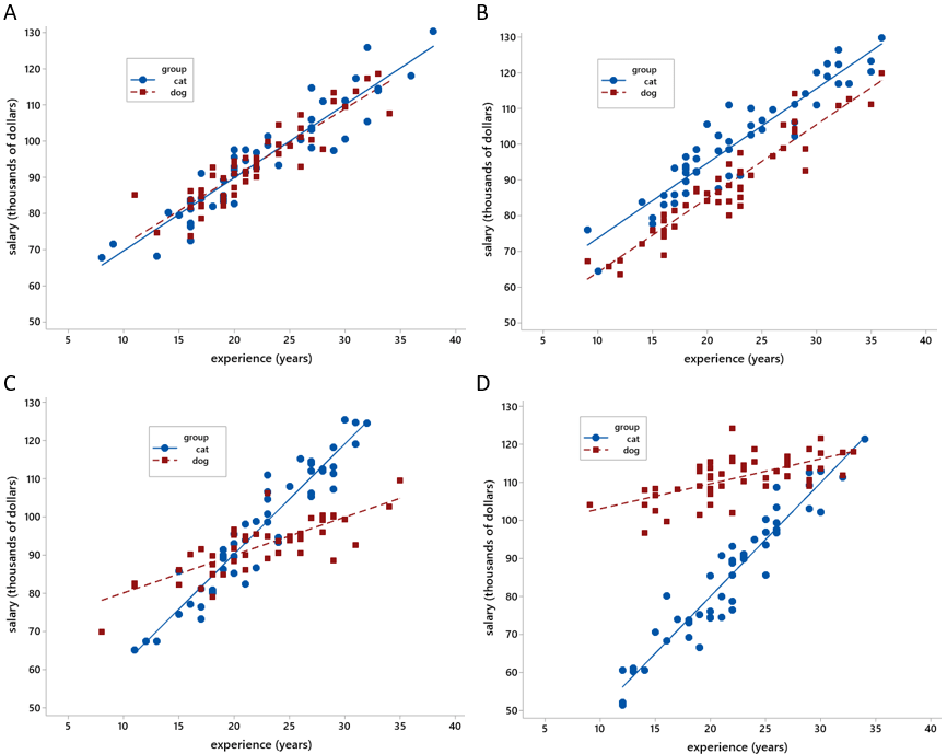
A free-response question for students is: Describe the relationship between salary and experience at each company. Also describe how the relationship varies (if at all) with regard to whether the employee works with cats or dogs. Reading and grading their responses can take a while, though. A multiple-choice version could present students with four descriptions and ask them to match each description to a graph. Here are some descriptions:
- (a) Salary increases much more quickly, for each additional year of experience, for cat lovers than for dog lovers. But dog lovers start out with much higher salaries than cat lovers, so much that it takes a bit more than 30 years of experience for cat lovers to catch up.
- (b) Salary increases by about $2000 for each additional year of experience, essentially the same for both cat and dog lovers, but cat lovers earn about $10,000 more than dog lovers at every experience level.
- (c) Salary increases by about $2000 for each additional year of experience, essentially the same for both cat and dog lovers.
- (d) Salary increases much more quickly, for each additional year of experience, for cat lovers than for dog lovers. Cat lovers generally earn less than dog lovers if they have less than about 20 years of experience, but cat lovers generally earn more than dog lovers beyond 20 years of experience.
Which graph goes with which description? (a): Graph D; (b): Graph B; (c): Graph A; (d): Graph C
Multivariable thinking is a core component of statistical thinking. The 2016 GAISE recommendations (here) explicitly called for introductory students to experience multivariable thinking in a variety of contexts. I think this example about smoking and lung capacity provides a rich context for such a learning activity. The surprising aspect of the initial finding captures students’ attention, and the resulting explanation involving age is both understandable and comforting.
Statistics and data truly can illuminate important questions about the world. Introductory students can experience this on the first day of class.
P.S. Michael Kahn wrote about this dataset for Stats magazine in 2003, when Beth Chance and I edited that magazine, and also for the Journal of Statistics Education in 2005 (here). The JSE article describes the source of the data and also contains a link to the datafile (near the end of the article).
A recent JSE article (here), written by Kevin Cummiskey and co-authors, uses this dataset for introducing students to causal inference.
De Veaux’s article and dataset about the worth of a fireplace can be found among ASA’s Stats 101 resources (here). This example is also mentioned in the 2016 GAISE report (here).
Minitab statistical software (here) was used to produce the graphs in this post.


Trackbacks & Pingbacks