#32 Create your own example, part 2

In last week’s post (here), I presented examples of questions that ask students to create their own example that satisfies a particular property, such as the mean exceeding the mean and inter-quartile range equaling zero.  I proposed that such questions can help students to think more carefully and deepen their understanding of statistical concepts.  All of last week’s examples concerned descriptive statistics.

Now I extend this theme to the realm of statistical inference concepts and techniques.  I present six create-your-own-example questions (each with multiple parts) concerning hypothesis tests and confidence intervals for proportions and means, with a chi-square test appearing at the end.  I believe these questions lead students to develop a stronger understanding of concepts such as the role of sample size and sample variability on statistical inference.

I encourage students to use technology, such as the applet here, to calculate confidence intervals, test statistics, and p-values.   This enables them to focus on underlying concepts rather than calculations.

The numbering of these questions picks up where the previous post left off.  As always, questions for students appear in italics.

---

6. Suppose that you want to test the null hypothesis that one-third of all adults in your county have a tattoo, against a two-sided alternative.  For each of the following parts, create your own example of a sample of 100 people that satisfies the indicated property.  Do this by providing the sample numbers with a tattoo and without a tattoo.  Also report the test statistic and p-value from a one-proportion z-test.

• a) The two-sided p-value is less than 0.001.
• b) The two-sided p-value is greater than 0.20.

Students need to realize that sample proportions closer to one-third produce larger p-values, while those farther from one-third generate smaller p-values.  Clever students might give the most extreme answers, saying that all 100 have a tattoo in part (a) and that 33 have a tattoo in part (b).

Instead of asking for one example in each part, you could make the question more challenging by asking students to determine all possible sample values that satisfy the property.  It turns out that for part (a), the condition is satisfied by having 17 or fewer, or 49 or more, with a tattoo.  For part (b), having 28 to 39 (inclusive) with a tattoo satisfies the condition.  Instead of trial-and-error, you could ask students to determine these values algebraically from the z-test statistic formula, but I would only ask this in courses for mathematically inclined students.

---

7. Suppose that you want to estimate the proportion of all adults in your county who have a tattoo. For each of the following parts, create your own example to satisfy the indicated property.  Do this by specifying the sample size and the number of people in the sample with a tattoo.  Also determine the confidence interval.

• a) The sample proportion with a tattoo is 0.30, and a 95% confidence interval for the population proportion includes the value 0.35.
• b) The sample proportion with a tattoo is 0.30, and a 99% confidence interval for the population proportion does not include the value 0.35.

The key here is to understand the impact of sample size on a confidence interval.  The confidence interval in both parts will be centered at the value of the sample proportion value of 0.30, so the interval in part (b) needs to be narrower than the interval in part (a).  A larger sample size produces a narrower confidence interval, so a smaller sample size is needed in part (a).

One example that works for part (a) is a sample of 100 people, 30 of whom have a tattoo, for part (a), which produces a 95% confidence interval of (0.210 → 0.390).  Similarly, creating a sample of 1000 people, 300 of whom have a tattoo, satisfies part (b), as the 99% confidence interval is (0.263 → 0.337).

Again you could consider asking students to determine all sample sizes that work.  Restricting attention to multiples of 10 (so the sample proportion with a tattoo equals 0.30 exactly), it turns out that a sample size of 340 or fewer suffices for part (a), and a sample size of 560 or more is needed for part (b).

 

---

8. Suppose that you want to estimate the population mean body temperature of a healthy adult with a 95% confidence interval.  For each of the following parts, create your own example of a sample of 10 body temperature values that satisfy the indicated property.  Do this by listing the ten values and also producing a dotplot that displays the ten values.  Report the sample standard deviation, and determine the confidence interval.

• a) The sample mean is 98.0 degrees, and a 95% confidence interval for the population mean includes the value 98.6.
• b) The sample mean is 98.0 degrees, and a 99% confidence interval for the population mean does not include the value 98.6.

This question is similar to the previous one, but dealing with a mean instead of a proportion brings the variability of the sample data into consideration.  This question removes sample size from consideration by stipulating that n = 10. 

The confidence interval for both parts will be centered at the value of the sample mean temperature: 98.0 degrees.  For the confidence interval in part (a) to include the value 98.6, the sample data need to display a good bit of variability.  A student might try a fairly simple example containing five values of 97.0 and five values of 99.0, which produces a sample standard deviation of 1.054 and a 95% confidence interval of (96.92 → 99.08) degrees.

In contrast, part (b) requires less sample variability, for the confidence interval to fall short of the value 98.6.  A student might use a fairly extreme example, such as one value of 97.9, eight values of 98, and one value of 98.1.  This results in a sample standard deviation of 0.047 and a 99% confidence interval of (97.95 → 98.05) degrees.

As with the previous questions, you could ask students to determine all values of the sample standard deviation that will work, either with trial-and-error or algebraically.  It turns out that the sample standard deviation needs to be at least 0.839 (to three decimal places) degrees in part (a), at most 0.583 degrees in part (b).

---

9. Suppose that you ask dog and cat owners whether their pet has been to a veterinarian in the past twelve months.  You organize the resulting counts in a 2×2 table as follows:

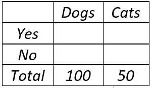
For each of the following parts, create your own example of a sample that satisfies the indicated property.  Do this by filling in the counts of the 2×2 table.  Also report the two sample proportions and the test statistic and p-value from a two-proportions z-test.

• a) The two-sided p-value is less than 0.001.
• b) The two-sided p-value is between 0.2 and 0.6.

Students need to produce a large difference in proportions for part (a) and a fairly small difference for part (b).  They could give a very extreme answer in part (a) by having 100% of dogs and 0% of cats visit a veterinarian.  A less extreme response that 80 of 100 dogs and 20 of 50 cats have been to a veterinarian produces a z-statistic of 4.90 and a p-value very close to zero.   

Stipulating that the p-value in part (b) must be less than 0.6 forces students not to use identical success proportions in the two groups.  One example that works is to have 80 of 100 dogs and 36 of 50 cats with a veterinarian visit. This produces a z-statistic of 1.10 and a p-value of 0.270.

---

10. The Gallup organization surveyed American adults about how many times they went to a movie at a movie theater in the year 2019.  They compared results for people with at least one child under age 18 in their household and those without such a child in their household.  Suppose that you reproduce this study by interviewing a random sample of adults in your county, and suppose that the sample means are the same as in the Gallup survey: 6.8 movies for those with children, 4.7 movies for those without, as shown in the table below:

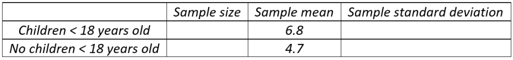
For each of the following parts, create your own example that satisfies the indicated property.  Do this by filling in the sample size and sample standard deviation for each group.  Also report the value of the two-sample t-test statistic and the two-sided p-value.

• a) The two-sample t-test statistic is less than 1.50.
• b) The two-sample t-test statistic is greater than 2.50.

Students have considerable latitude in their answers here, as they can focus on sample size or sample variability.  They need to realize that large sample sizes and small standard deviations will generally produce larger test statistic values, as for part (a).  To produce a smaller test statistic value in part (b) requires relatively small sample sizes or large standard deviations.

For example, sample sizes of 10 and sample standard deviations of 4.0 for each group produce t = 1.17 to satisfy part (a).  The condition for part (b) can be met with the same standard deviations but larger sample sizes of 50 for each group, which gives t = 2.62.

---

11. Suppose that you interview a sample of 100 adults, asking for their political viewpoint (classified as liberal, moderate, or conservative) and how often they eat ice cream (classified as rarely, sometimes, or often).  Also suppose that you obtain the marginal totals shown in the following 3×3 table:

For each of the following parts, create your own example that satisfies the indicated property.  Do this by filling in the counts of the 3×3 table.  Also report the value of the chi-square statistic and p-value.  For part (b), also describe the nature of the association between the variables (i.e., which political groups tend to eat ice cream more or less frequently?).

• b) The chi-square p-value is between 0.4 and 0.8.
• c) The chi-square p-value is less than 0.001.

Like the previous questions, this one also affords students considerable leeway with their responses.  They need to supply nine cell counts in the table, but the fixed margins mean that they only have four degrees of freedom* to play around with.

* Once a student has filled in four cell counts (provided that they are not all in the same row or same column), the other five cell counts are then determined by the need to make counts add up to the marginal totals.

First students need to realize that to obtain a large p-value in part (a), the counts need to come close to producing independence between political viewpoint and ice cream frequency.  They also need to know that independence here would mean that all three political groups have 20% rarely, 50% sometimes, and 30% often eating ice cream.  Independence would produce this table of counts:

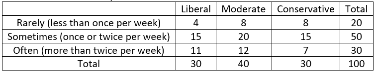
This table does not satisfy the condition for part (a), though, because the p-value is 1.0.  A correct response to part (a) requires a bit of variation from perfect independence.  The following table, which shifts two liberals from rarely to often and two conservatives from often to rarely, produces a chi-square statistic of 2.222 and a p-value of 0.695:

On the other hand, a table that successfully satisfies part (b) needs to reveal a clear association between the two variables.  Consider the following example:

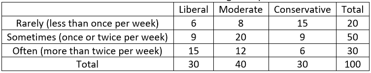
The chi-square test statistic equals 13.316 for this example, and the p-value is 0.010.  This table reveals that makes liberals much more likely to eat ice cream often, and much less likely to eat ice cream rarely, compared to conservatives.

---

Students can use create-your-own-example questions to demonstrate and deepen their understanding of statistical concepts.  The previous post provided many examples that concerned descriptive statistics, and this post has followed suit with topics of statistical inference.

I also like to ask create-your-own-example questions that ask students, for instance, to identify a potential confounding variable in a study, or to suggest a research question for which comparative boxplots would be a relevant graph.  Perhaps a future post will discuss those kinds of questions.

As with the previous post, I leave you with a (completely optional, of course) take-home assignment: Create your own example of a create-your-own-example question to ask of your students.

P.S. A recent study (discussed here) suggests that average body temperature for humans, as discussed in question 8, has dropped in the past century and is now close to 97.5 degrees Fahrenheit.  The Gallup survey mentioned in question 10 can be found here.