#13 A question of trust
Which do you trust more: a simulation-based* or normal-based analysis of an inference question? In other words, if a simulation analysis and normal approximation give noticeably different p-values, which would you believe to be closer to the correct p-value? Please think about this question in the abstract for a moment. Soon we’ll come back to it in specific example.
* If you’re not familiar with simulation-based inference, I recommend reading post #12 (here) first.
Here’s the example that we’ll consider throughout this post: Stemming from concern over childhood obesity, researchers investigated whether children might be as tempted by toys as by candy for Halloween treats (see abstract of article here). Test households in five Connecticut neighborhoods offered two bowls to trick-or-treating children: one with candy and one with small toys. For each child, researchers kept track of whether the child selected the candy or the toy. The research question was whether trick-or-treaters are equally likely to select the candy or toy. More specifically, we will investigate whether the sample data provide strong evidence that trick-or-treaters have a tendency to select either the candy or toy more than the other.
In my previous post (here) I argued against using terminology and formalism when first introducing the reasoning process of statistical inference. In this post I’ll assume that students have now been introduced to the structure of hypothesis tests, so we’ll start with a series of background questions before we analyze the data (my questions to students appear in italics):
- What are the observational units? The trick-or-treaters are the observational units.
- What is the variable, and what type of variable is it? The variable is the kind of treat selected by the child: candy or toy. This is a binary, categorical variable.
- What is the population of interest? The population is all* trick-or-treaters in the U.S. Or perhaps we should restrict the population to all trick-or-treaters in Connecticut, or in this particular community.
- What is the sample? The sample is the trick-or-treaters in these Connecticut neighborhoods whose selections were recorded by the researchers.
- Was the sample selected randomly from the population? No, it would be very difficult to obtain a list of trick-or-treaters from which one could select a random sample. Instead this is a convenience sample of trick-or-treaters who came to the homes that agreed to participate in the study. We can hope that these trick-or-treaters are nevertheless representative of a larger population, but they were not randomly selected from a population.
- What is the parameter of interest? The parameter is the population proportion of all* trick-or-treaters who would select the candy if presented with this choice between candy and toy. Alternatively, we could define the parameter to be the population proportion who would select the toy. It really doesn’t matter which of the two options we designate as the “success,” but we do need to be consistent throughout our analysis. Let’s stick with candy as success.
- What is the null hypothesis, in words? The null hypothesis is that trick-or-treaters are equally likely to select the candy or toy. In other words, the null hypothesis is that 50% of all trick-or-treaters would select the candy.
- What is the alternative hypothesis, in words? The alternative hypothesis is that trick-or-treaters are not equally likely to select the candy or toy. In other words, the alternative hypothesis is that the proportion of all trick-or-treaters who would select the candy is not 0.5. Notice that this is a two-sided hypothesis.
- What is the null hypothesis, in symbols? First we have to decide what symbol to use for a population proportion. Most teachers and textbooks use p, but I prefer to use π. I like the convention of using Greek letters for parameters (such as μ for a population mean and σ for a population standard deviation), and I see no reason to abandon that convention for a population proportion. Some teachers worry that students will immediately think of the mathematical constant 3.14159265… when they see the symbol π, but I have not found this to be a problem. The null hypothesis is H0: π = 0.5.
- What is the alternative hypothesis, in symbols? The two-sided alternative hypothesis is Ha: π ≠ 0.5.
* I advise students that it’s always a nice touch to insert the word “all” when describing a population and parameter.
Whew, that was a lot of background questions! Notice that I have not yet told you how the sample data turned out. I think it’s worth showing students that the issues above can and should be considered before looking at the data. So, how did the data turn out? The researchers found that 148 children selected the candy and 135 selected the toy. The value of the sample proportion who selected the candy is therefore 148/283 ≈ 0.523.
Let’s not lose sight of the research question here: Do the sample data provide strong evidence that trick-or-treaters have a tendency to select either the candy or toy more than the other? To pursue this I ask: How can we investigate whether the observed value of the sample statistic (.523 who selected the candy) would be very surprising under the null hypothesis that trick-or-treaters are equally likely to select the candy or toy? I hope that my students will erupt in a chorus of, “Simulate!”*
* I tell my students that if they ever drift off to sleep in class and are startled awake to find that I have called on them with a question, they should immediately respond with: Simulate! So many of my questions are about simulation that there’s a reasonable chance that this will be the correct answer. Even if it’s not correct, I’ll be impressed.
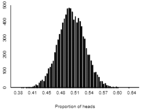
Here is a graph of the distribution of sample proportions resulting from 10,000 repetitions of 283 coin flips (using the One Proportion applet here):

I ask students: Describe the shape, center, and variability of the distribution of these simulated sample proportions. The shape is very symmetric and normal-looking. The center appears to be near 0.5, which makes sense because our simulation assumed that 50% of all children would choose the candy. Almost all of the sample proportions fall between 0.4 and 0.6, and it looks like about 90% of them fall between 0.45 and 0.55.
But asking about shape, center, and variability ignores the key issue. Next I ask this series of questions:
- What do we look for in the graph, in order to assess the strength of evidence about the research question? We need to see whether the observed value of the sample statistic (0.523) is very unusual.
- Well, does it appear that 0.523 is unusual? Not unusual at all. The simulation produced sample proportions as far from 0.5 as 0.523 fairly frequently.
- So, what do we conclude about the research question, and why? The sample data (0.523 selecting the candy) would not be surprising if children were equally likely to choose the candy or toy, so the data do not provide enough evidence to reject the (null) hypothesis that children are equally likely to choose the candy or toy.
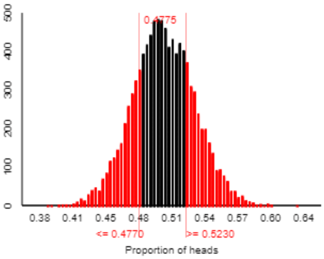
We could stop there, absolutely. We don’t need to calculate a p-value or anything else in order to draw this conclusion. We can see all we need from the graph of simulation results. But let’s go ahead and calculate the (approximate) p-value from the simulation. Because we have a two-sided alternative, a sample proportion will be considered as “extreme” as the observed one if it’s at least as far from 0.5 as 0.523 is. In other words, the p-value is the probability of obtaining a sample proportion of 0.477 or less, or 0.523 or more, if the null hypothesis were true. The applet reveals that 4775 of the 10,000 simulated sample proportions are that extreme, as shown in red below:

The approximate p-value from the simulation analysis is therefore 0.4775. This p-value is nowhere near being less than 0.05 or 0.10 or any reasonable significance level, so we conclude that the sample data do not provide sufficient evidence to reject the null hypothesis that children are equally likely to choose the candy or toy.
When I first asked about how to investigate the research question, you might have been thinking that we could use a normal approximation, also known as a one-proportion z-test. Let’s do that now: Apply a one-proportion z-test to these data, after checking the sample size condition. The condition is certainly satisfied: 283(.5) = 141.5 is far larger than 10. The z-test statistic can be calculated as:

This z-score tells us that the observed sample proportion who selected candy (0.523) is less than one standard deviation away from the hypothesized value of 0.5. The two-sided p-value from the normal distribution to be ≈ 2×0.2198 = 0.4396. Again, of course, the p-value is not small and so we conclude that the sample data do not provide sufficient evidence to reject the null hypothesis of equal likeliness.
But look at the two p-values we have generated: 0.4775 and 0.4396. Sure, they’re in the same ballpark, but they’re noticeably different. On a percentage basis, they differ by 8-9%, which is non-trivial. Which p-value is correct? This one is easy: Neither is correct! These are both approximations.
Finally, we are back to the key question of the day, alluded to the title of this post and posed in the first paragraph: Which do you trust more: the (approximate) p-value based on simulation, or the (approximate) p-value based on the normal distribution? Now that we have a specific example with two competing p-values to compare, please think some more about your answer before you read on.
Many students (and instructors) place more trust in the normal approximation. One reason for this is that the normal distribution is based on a complicated formula and sophisticated mathematics. Take a look at the probability density function* of a normal distribution:

* Oh dear, I must admit that in this expression the symbol π does represent the mathematical constant 3.14159265….
How could such a fancy-looking formula possibly go wrong? More to the point, how could this sophisticated mathematical expression possibly do worse than simulation, which amounts to just flipping a coin a whole bunch of times?
An even more persuasive argument for trusting the normal approximation, in many students’ minds, is that everyone gets the same answer if they perform the normal-based method correctly. But different people get different answers from a simulation analysis. Even a single person gets different answers if they conduct a simulation analysis a second time. This lack of exact replicability feels untrustworthy, doesn’t it?
So, how can we figure out which approximation is better? Well, what does “better” mean here? It means closer to the actual, exact, correct p-value. Can we calculate that exact, correct p-value for this Halloween example? If so, how? Yes, by using the binomial distribution.
If we let X represent a binomial distribution with parameters n = 283 and π = 0.5, the exact p-value is calculated as Pr(X ≤ 135) + Pr(X ≥ 148)*. This probability turns out (to four decimal places) to be 0.4757. This is the exact p-value, to which we can compare the approximate p-values.
* Notice that the values 135 and 148 are simply the observed number who selected toy and candy, respectively, in the sample.
So, which approximation method does better? Simulation-based wins in a landslide over normal-based:

This is not a fluke. With 10,000 repetitions, it’s not surprising that the simulation-based p-value* came so close to the exact binomial p-value. The real question is why the normal approximation did so poorly, especially in this example where the validity conditions were easily satisfied, thanks to a large sample size of 283 and a population proportion of 0.5.
* I promise that I only ran the simulation analysis once; I did not go searching for a p-value close to the exact one. We could also calculate a rough margin-of-error for the simulation-based p-value to be about 1/sqrt(10,000) ≈ .01.
The problem with the normal approximation, and a method for improving it, go beyond the scope of a typical Stat 101 course, but I do present this in courses for mathematically inclined students. First think about it: Why did the normal approximation do somewhat poorly here, and how might you improve the normal approximation?
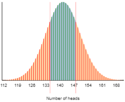
The problem lies in approximating a discrete probability distribution (binomial) with a continuous one (normal). The exact binomial probability is the sum of the heights of the red segments in the graph below, whereas the normal approximation calculates the area under the normal curve to the left of 135 and the right of 148:

The normal approximation can be improved with a continuity correction, which means using 135.5 and 147.5, rather than 135 and 148, as the endpoints for the area under the curve. This small adjustment leads to including a bit more of the area under the normal curve. The continuity-corrected z-score becomes 0.713 (compared to 0.773 without the correction) and the two-sided normal-based p-value (to four decimal places) becomes 0.4756, which differs from the exact binomial p-value by only 0.0001. This seemingly minor continuity correction greatly improves the normal approximation to the binomial distribution.
My take-away message is not that normal-based methods are bad, and also not that we should teach the continuity correction to introductory students. My point is that simulation-based inference is good! I think many teachers regard simulation as an effective tool for studying concepts such as sampling distributions and for justifying the use of normal approximations. I agree with this use of simulation wholeheartedly, as far as it goes. But we can help our students to go further, recognizing that simulation-based inference is very valuable (and trustworthy!) in its own right.

Trackbacks & Pingbacks