#29 Not enough evidence

We statistics teachers often ask students to draw a conclusion, in the context of the data and research question provided, from the p-value of a hypothesis test.  Do you think a student is more likely to provide a response that earns full credit if the p-value is .02 or .20?

You may respond that it doesn’t matter.  You may believe that a student either knows how to state a conclusion from a p-value or not, regardless of whether the p-value is small or not-so-small.

I think it does matter, a lot.  I am convinced that students are more likely to give a response that earns full credit from a small p-value like .02 than from a not-so-small p-value like .20.  I think it’s a lot easier for students to express a small p-value conclusion of strong evidence against the null than a not-so-small p-value conclusion of not much evidence against the null.  Why?  In the not-so-small p-value case, it’s very easy for students to slip into wording about evidence for the null hypothesis (or accepting the null hypothesis), which does not deserve full credit in my book.

In this post I will explore this inclination to mis-state hypothesis test conclusions from a not-so-small p-value.  I will suggest two explanations for convincing students that speaking of evidence for the null, or deciding to accept the null, are not appropriate ways to frame conclusions.  I will return to an example that we’ve seen before and then present two new examples.  As always, questions that I pose to students appear in italics.

---

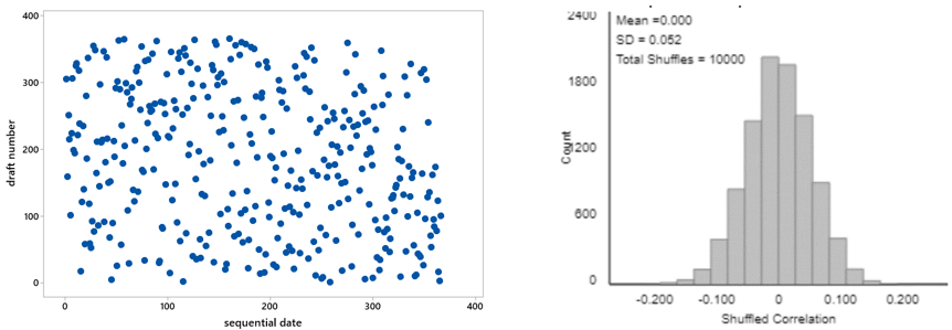
Let’s revisit the infamous 1970 draft lottery, which I discussed in post #9 (Statistics of illumination, part 3, here).  To recap: All 366 birthdays of the year were assigned a draft number.  The scatterplot on the left below displays the draft numbers vs. sequential day numbers.  At first glance, the graph appears to show nothing but random scatter, as we would expect from a truly random lottery.  But when we explored the data further, we found a bit of negative association between draft number and day number, with a correlation coefficient of -0.226.  We used simulation to investigate how surprising such a correlation would be with a truly random lottery.  The graph on the right shows the results for 10,000 random lotteries.  We see that none of the 10,000 simulated correlation coefficients is as large (in absolute value) as the -0.226 value that was achieved with the actual 1970 draft lottery.  Therefore, because a result as extreme as the one observed would be very unlikely to occur with a truly random lottery, we concluded that the observed data provide very strong evidence that the lottery process was not truly random.  (The explanation turned out to be insufficient mixing of the capsules containing the birthdays.)

This reasoning process is by no means trivial, but I think it makes sense to most students.  Without using the terminology, we have conducted a hypothesis test.  The null hypothesis is that the lottery process was truly random.  The alternative hypothesis is that the process was not truly random.  The p-value turns out to be very close to zero, less than 1 in 10,000.  Therefore, we have very strong evidence against the null hypothesis in favor of the alternative.

In the following year’s (1971) draft lottery, additional steps were taken to try to produce a truly random process.  The correlation coefficient (between draft number and day number) turned out to be 0.014.  The graph of simulation results above* shows that such a correlation coefficient is not the least bit unusual or surprising if the lottery process was truly random.  The two-sided p-value turns out to be approximately 0.78.  What do you conclude about the 1971 lottery process?

* This 1971 draft lottery involved 365 birthdays, as compared to 366 birthdays in the 1970 draft lottery.  This difference is so negligible that using the same simulation results is reasonable.

After they provide their open-ended response, I also ask students: Which of the following responses are appropriate and which are not?

• A: The data do not provide enough evidence to conclude that the 1971 lottery process was not truly random.
• B: The data do not provide much evidence for doubting that the 1971 lottery process was truly random.
• C: The data provide some evidence that the 1971 lottery process was truly random.
• D: The data provide strong evidence that the 1971 lottery process was truly random.

Responses A and B are correct and appropriate.  But they are challenging for students to express, in large part because they include a double negative.  It’s very tempting for students to avoid the double negative construction and write a more affirmative conclusion. But the affirmative responses (C and D) get the logic of hypothesis testing wrong by essentially accepting the null hypothesis.  That’s a no-no, so those responses deserve only partial credit in my book.

Students naturally ask: Why is this wrong?  Very good question.  I have two answers, one fairly philosophical and the other more practical.  I will lead off with the philosophical answer, even though students find the practical answer to be more compelling and persuasive.

---

The philosophical answer is: Accepting a null hypothesis, or assessing evidence in favor of the null hypothesis, is simply not how the reasoning process of hypothesis testing works.  The reasoning process only assesses the strength of evidence that the data provide against the null hypothesis.  Remember how this goes: We start by assuming that the null hypothesis is true.  Then we see how surprising the observed data would be if the null hypothesis were true.  If the answer is that the observed data would be very surprising, then we conclude that the data provide strong evidence against the null hypothesis.  If the answer is that the observed data would be somewhat surprising, then we conclude that the data provide some evidence against the null hypothesis.  But what if the answer is that the observed data would not be surprising?  Well, then we conclude that the data provide little or no evidence against the null hypothesis.

This reasoning process is closely related to the logical argument called modus tollens:

• If P then Q
• Not Q
• Therefore: not P

For example, the Constitution of the United States stipulates that if a person is eligible to be elected President in the year 2020 (call this P), then that person must have been born in the U.S. (call this Q).  We know that Queen Elizabeth was not born in the U.S. (not Q).  Therefore, Queen Elizabeth is not eligible to be elected U.S. President in 2020 (not P).

But what if Q is true?  The following, sometimes called the fallacy of the converse, is NOT VALID:

• If P then Q
• Q
• Therefore: P

For example, Taylor Swift was born in the U.S. (Q).  Does this mean that she is eligible to be elected President in 2020 (P)?  No, because she is younger than 35 years old, which violates a constitutional requirement to serve as president.

For the draft lotteries, P is the null hypothesis that the lottery process was truly random, and Q is that the correlation coefficient (between day number and draft number) is between about -0.1 and 0.1.  Notice that (If P, then Q) is not literally true here, but P does make Q very likely.  This is the stochastic* version of the logic.  For the 1970 lottery, we observed a correlation coefficient (-0.226) that is not Q, so we have strong evidence for not P, that the lottery process was not truly random.  For the 1971 lottery, we obtained a correlation coefficient (0.014) that satisfies Q.  This leaves us with no evidence for not P (that the lottery process was non-random), but we also cannot conclude P (that the lottery process was random).

* I don’t use this word with introductory students.  But I do like the word stochastic, which simply means involving randomness or uncertainty.

I only discuss modus tollens in courses for mathematics and statistics majors.  But for all of my students I do mention the common expression: Absence of evidence does not constitute evidence of absence.  For the 1971 draft lottery, the correlation coefficient of 0.014 leaves us with an absence of evidence that anything suspicious (non-random) was happening, but that’s not the same as asserting that we have evidence that nothing suspicious (non-random) was happening.

---

My second answer, the more practical one, for why it’s inappropriate to talk about evidence in favor of a null hypothesis, or to accept a null hypothesis, is: Many different hypotheses are consistent with the observed data, so it’s not appropriate to accept any one of these hypotheses.  Let me use a new example to make this point.

Instead of flipping a coin, tennis players often determine who serves first by spinning a racquet and seeing whether it lands with the label facing up or down.  Is this really a fair, 50/50 process?  A student investigated this question by spinning her racquet 100 times, keeping track of whether it landed with the label facing up or down.

• a) What are the observational units and variable?  The observational units are the 100 spins of the racquet.  The variable is whether the spun racquet landed with the label facing up or down.  This is a binary, categorical variable.
• b) Identify the parameter of interest.  The parameter is the long-run proportion of all spins for which the racquet would land with the label up*.  This could also be expressed as the probability that the spun racquet would land with the label facing up.
• c) State the null and alternative hypotheses in terms of this parameter.  The null hypothesis is that the long-run proportion of all spins that land up is 0.5.  In other words, the null hypothesis states that racquet spinning is a fair, 50/50 process, equally likely to land up or down.  The alternative hypothesis is that the long-run proportion of all spins that land up is not 0.5.  This is a two-sided alternative.

* We could instead define a down label as a success and specify the parameter to be the long-run proportion of all spins that would land down.

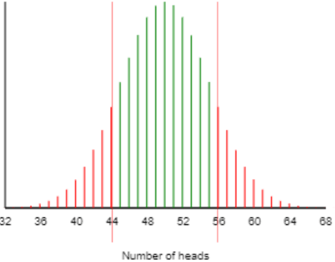
The 100 racquet spins in the sample resulted in 44 that landed with the label up, 56 that landed with the label down.  The two-sided p-value turns out to be 0.271, as shown in the following graph of a binomial distribution*:

* You could also (or instead) present students with an approximate p-value from a simulation analysis or a normal distribution.

• d) Interpret this p-value.  If the racquet spinning process was truly fair (equally likely to produce an up or down result), there’s a 27.1% chance that a random sample of 100 spins would produce a result as extreme as the actual one: 44 or fewer, or 56 or more, spins landing with the label up.
• e) Summarize your conclusion.  The sample data (44 landing up in 100 spins) do not provide much evidence against the hypothesis that racquet spinning is a fair, 50/50 process.
• f) Explain how your conclusion follows from the p-value.  The p-value of 0.271 is not small, indicating that the observed result (44 landing up in 100 spins), or a result more extreme, would not be surprising if the racquet spinning process was truly fair.  In other words, the observed result is quite consistent with a fair, 50/50 process.

Once again this conclusion in part (e) is challenging for students to express, as it involves a double negative.  Students are very tempted to state the conclusion as: The sample data provide strong evidence that racquet spinning is a fair, 50/50 process.  Or even more simply: Racquet spinning is a fair, 50/50 process.

To help students understand what’s wrong with these conclusions, let’s focus on the parameter, which is the long-run proportion of racquet spins that would land with the label facing up.  Concluding that racquet spinning is a fair, 50/50 process means concluding that the value of this parameter equals 0.5. 

I ask students: Do we have strong evidence against the hypothesis that 45% of all racquet spins would land up?  Not at all!  This hypothesized value (0.45) is very close to the observed value of the sample proportion of spins that landed up (0.44).  The p-value for testing the null value of 0.45 turns out to be 0.920*.

* All of the p-values reported for this example are two-sided, calculated from the binomial distribution.

Let’s keep going: Do we have strong evidence against the hypothesis that 40% of all racquet spins would land up?  Again the answer is no, as the p-value equals 0.416.  What about 52%?  Now the p-value is down to 0.111, but that’s still not small enough to rule out 0.52 as a plausible value of the parameter.

Where does this leave us?  We cannot reject that the racquet spinning process is fair (parameter value 0.5), but there are lots and lots* of other parameter values that we also cannot reject.  Therefore, it’s inappropriate to accept one particular value, or to conclude that the data provide evidence in favor of one particular value, because there are many values that are similarly plausible for the parameter.  The racquet spinning process might be fair, but it also might be biased slightly in favor of up or considerably against up.

* Infinitely many, in fact

---

Now let’s consider a new example, which addresses the age-old question: Is yawning contagious?  The folks at the popular television series MythBusters investigated this question by randomly assigning 50 volunteers to one of two groups:

• Yawn seed group: A confederate of the show’s hosts purposefully yawned as she individually led 34 subjects into a waiting room.
• Control group: The person led 16 other subjects into a waiting room and was careful not to yawn.

All 50 subjects were observed by hidden camera as they sat in the room, to see whether or not they yawned as they waited for someone to come in.  Here is the resulting 2×2 table of counts:

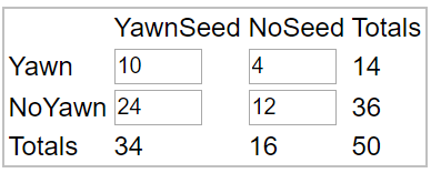
The hosts of the show calculated that 10/34 ≈ 0.294 of the subjects in the yawn seed group yawned, compared to 4/16 = 0.250 of the subjects in the control group.  The hosts conceded that this difference is not dramatic, but they noted that the yawn seed group had a higher proportion who yawned than the control group, and they went on declare that the data confirm the yawning is contagious hypothesis.

We can use an applet (here) to simulate a randomization test* on these data.  The p-value turns out to be approximately 0.513, as seen in the following graph of simulation results:

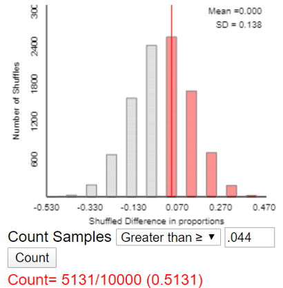
* See post #27 (Simulation-based inference, part 2, here) for an introduction to such an analysis.

• a) State the null and alternative hypothesis, in words.
• b) Do you agree with the conclusion reached by the show’s hosts? Explain.
• c) How would you respond to someone who concluded: “The hosts are completely wrong.  The data from this study actually provide strong evidence that yawning is not contagious.”

a) The null hypothesis is that yawning is not contagious.  In other words, the null hypothesis is that people exposed to a yawn seed group have the same probability of yawning as people not so exposed.  The alternative hypothesis is that yawning is contagious, so people exposed to a yawn seed group are more likely to yawn than people not so exposed.

b) The conclusion of the show’s hosts is not supported by the data.  Such a small difference in yawning proportions between the two groups could easily have occurred by the random assignment process alone, even if yawning is not contagious.  The data do not provide nearly enough evidence for concluding that yawning is contagious.

c) This conclusion goes much too far in the other direction.  It’s not appropriate to conclude that yawning is not contagious.  A hypothesis test only assesses evidence against a null hypothesis, not in favor of a null hypothesis.  It’s plausible that yawning is not contagious, but the observed data are also consistent with yawning being a bit contagious or even moderately contagious.

---

As I wrap up this lengthy post, let me offer five pieces of advice for helping students to avoid mis-stating conclusions from not-so-small p-values:

1. I strongly advise introducing hypothesis testing with examples that produce very small p-values and therefore provide strong evidence against the null hypothesis.  The blindsight study that I used in post #12 (Simulation-based inference, part 1, here) is one such example.  I think a very small p-value makes it much easier for students to hang their hat on the reasoning process behind hypothesis testing.

2. Later be sure to present several examples that produce not-so-small* p-values, giving students experience with drawing “not enough evidence to reject the null” conclusions.

* You have no doubt noticed that I keep saying not-so-small rather than large.  I think this also indicates how tricky it is to work with not-so-small p-values.  A p-value of .20 does not provide much evidence against a null hypothesis, and I consider a p-value of .20 to be not-so-small rather than large.

3. Emphasize that there are many plausible values of the parameter that would not be rejected by a hypothesis test, so it’s not appropriate to accept the one particular value that appears in the null hypothesis.

4. Take a hard line when grading students’ conclusions.  Do not give full credit for a conclusion that mentions evidence for a null hypothesis or accepts a null hypothesis.

5. In addition to asking students to state their own conclusions, provide them with a variety of mis-stated and well-stated conclusions, and ask them to identify which are which.

Do you remember the question that motivated this post? Are students more likely to earn full credit for stating a conclusion from a p-value of .02 or .20?  Are you persuaded to reject the hypothesis that students are equally likely to earn full credit with either option? Have I provided convincing arguments that drawing an appropriate conclusion is easier for students from a p-value of .02 than from a p-value of .20?