#6 Two dreaded words, part 1

Which two-word term produces more anxiety and negative feelings among introductory statistics students than any other?

I don’t think correlation coefficient produces the most negative feelings, or confidence interval, or even hypothesis test.  I don’t think random sample achieves maximum anxiety, or observational study, or expected value, or even confounding variable.  No, my bet is that standard deviation makes students shiver with fear and cringe with distaste more than any other two-word term, perhaps even long after they have completed their statistics course*.

Why is this so unfortunate?  Because variability is the single most fundamental concept in statistics, and the most common measure of variability is … (brace yourself) … standard deviation.

* If you would vote for sampling distribution, I see your point.  But I don’t think sampling distribution comes up outside of a statistics classroom nearly as much as standard deviation.  Trust me: I’ll have lots to say about teaching sampling distributions in later posts.

The formula for standard deviation (allow me to abbreviate this as SD for the rest of this post) can certainly look intimidating:

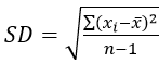
Expressing this as an algorithm does not make it any more palatable:

1. Subtract the mean from each data value.
2. Square each difference.
3. Add them up.
4. Divide by one less than the sample size.
5. Take the square root.

What to do?  I recommend asking questions that help students to understand what SD is all about, rather than wasting their time with calculating SD by hand.  Here are ten questions that try to do this:

1. Suppose that Samira records the ages of customers at the Snack Bar on a college campus from 12-2pm tomorrow, while Mary records the ages of customers at the McDonald’s near the highway at the same time.  Who will have the larger SD of their ages – Samira or Mary?  Explain why.

Mary is likely to encounter people of all ages at McDonald’s – from toddlers to senior citizens and every age in between.  Samira might run into some toddlers and senior citizens at the on-campus snack bar, but she’ll mostly find a lot of people in the 18-25-year-old age group.  Because the ages of McDonald’s customers will vary more than ages of Snack Bar customers, Mary will have a larger SD of ages than Samira will.

2. Suppose that Carlos and Hector visit their local humane society animal shelter.  Carlos records the weights of the 25 cats that they find there, and Hector records the weights of the 25 human beings that they encounter.  Who will have the larger SD of their weights – Carlos or Hector?

This question is getting at the same understanding as the previous one*. Most students are quick to realize that the weights of human beings vary much more than the weights of ordinary domestic cats, so Hector will have a larger SD than Carlos.

* But this question involves cats, and I like cats!  I plan to devote a future post to nothing but questions that involve cats in one way or another.

3. Draw four rectangles so that the SD of their widths is greater than the SD of their heights.  This question was sent to me by Camille Fairbourn and John Keane in their proposal to conduct a breakout session at the 2019 U.S. Conference on Teaching Statistics* (link).  They later told me that the original source for the question is the Illustrative Mathematics project (link). I especially like this question because if you understand the concept of SD, you can answer this question correctly with a moment’s thought and less than a minute of time to draw the rectangles.  But if you do not understand the concept, you’re not going to succeed by (accidentally) drawing the rectangles correctly by random chance.

* If you want to impress me with a proposal for a session in a conference that I am chairing: Ask good questions!

4. Consider the following dotplots of customer ratings (on a scale of 1 – 5) of four restaurants (A – D).  Arrange the four restaurants in order from smallest SD to largest SD, without performing any calculations.

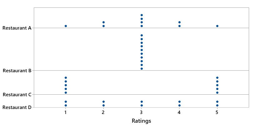
First notice that all four restaurants have an average (mean) rating of 3, right in the middle of the scale.  I hope that this helps students to focus on variability as the key idea here.

Let’s start with ratings of restaurant B, which display no variability whatsoever, because all 10 customers gave a mediocre rating of 3.  On the other extreme, customers disagree very strongly about restaurant C, with half giving a stellar rating of 5 and the other half giving a lousy rating of 1.  These extreme cases reveal that the SD is smallest for B and largest for C.

What about restaurants A and D?  Remember that the average (mean) rating is 3 for both, and notice that A has more ratings near the middle while D has more ratings on the ends.  In fact, you could produce the distribution for A by starting with D and moving one of the 1s and one of the 5s to 3.  Therefore, the SD is smaller for A than for D.   The correct ordering, from smallest SD to largest SD, is: B – A – D – C.

Many students struggle with this question, even when I encourage them to discuss it in groups.  I think one of their primary difficulties is appreciating that I am asking about the variability in the ratings.  Some students seem to think that the question is about variability in the frequencies (counts), so they think D shows no variability because the frequency is the same for each rating score (2 customers gave each possible rating score from 1 – 5).  Other students seem to think that variability refers to the number of different rating scores used, so they think that A has more variability than C because A’s customers used all five ratings scores whereas C’s customers only used the values 1, 3, and 5.

If you’re really intent on having students calculate an SD or two by hand, you might do that for the ratings of restaurants B and C here.  The calculation is very easy for B, because every customer gave a rating of 3, so the mean is 3, so all of the deviations from the mean are 0, so the SD = 0.  For restaurant C, the five ratings of 5 all have a squared deviation of 2² = 4, and the five ratings of 1 all have a squared deviation of (-2)² = 4.  The sum of squared deviations is therefore 10×4 = 40.  Dividing by one less than the sample size gives 40/9 ≈ 4.444.  Taking the square root gives SD ≈ 2.108.  We often say the SD “sorta-kinda” represents a typical deviation from the mean, so close to 2 seems about right for the SD of ratings in restaurant C.

The numerical values of these SDs turn out to be 0.000 for B, 1.115 for A, 1.491 for D, and 2.108 for C.

5. Now let’s throw a fifth restaurant into the mix.What about the SD of ratings for restaurant E below – where does that fall in the ordering among restaurants A-D?

Some students are fooled by the “bumpiness” of the distribution of ratings for restaurant E, because the frequencies/counts bounce up from a rating of 1 to a rating of 2, and then down to a rating of 3, and then back up to 4 and back down to 5.  But as we noted above, we need to focus on the variability of the ratings, not the variability of the frequencies.  Restaurant E’s ratings have more variability than B’s and less than C’s, but how do they compare to A and D?  Notice that you could create E’s distribution from D’s by moving a rating of 1 to a rating of 2 and a rating of 5 to a rating of 4.  So, E has less variability than D.  But E has more variability than A, because you could also create E’s distribution from A’s by moving one rating of 3 to 2 and another rating of 3 to 4.  The SD of the ratings for restaurant E turns out to be 1.247.

6. Can SD ever equal zero?  Under what circumstances?

Sure.  All that’s needed for an SD to equal zero is for the data to display no variability whatsoever.  In other words, SD = 0 when all of the data values equal the same value, as we saw with ratings of restaurant B above.

7. Can SD ever be negative?  Under what circumstances?

No, an SD value can never be negative.  Data cannot have less than no variability, so 0 is the smallest possible value for an SD.  Mathematically, the formula for SD involves squaring deviations from the mean; those squared values can never be negative.

8. If I were to add 5 points to the exam score of every student in my class, would the SD of the exam scores increase, decrease, or remain the same?  Explain why.

Adding 5 points to every exam score would shift the distribution of scores to the right by 5 points, and it would increase the average (mean) score by 5 points.  But the amount of variability in the exam scores would not change, so the SD would not change.

9. If I were to double the exam score of every student in my class, would the SD of the exam scores increase, decrease, or remain the same?  Explain why.

Doubling the exam scores increase their variability, so the SD would increase*.  To be more precise, the SD would double.  If you’re teaching a course for mathematically inclined students, you could ask them to derive this result from the formula, but I don’t recommend that for students in a typical “Stat 101” course.

* Some of you may be thinking that if every student earned identical exam scores in the first place, then doubling the scores would not increase the SD, because the SD would still equal zero.

10. If I were to add 500 points to the exam score for one lucky student in my class, would the SD of the exam scores change very much?  Explain your answer.

Yes, such an incredibly extreme outlier would have a massive impact on the SD.  How can you tell?  Because the mean would be greatly affected by the enormous outlier, and so deviations from the mean would also be affected, and so squared deviations would be all the more affected.  In other words, SD is not at all resistant to outliers.

There you have it – ten questions to help students make sense of standard deviation.  But wait a minute – there’s no real data in any of these examples!  That’s a fair criticism, but I think these questions can nevertheless be effective for developing conceptual understanding (recommendation #2 in the GAISE report, link).  Of course, we can ask good questions that develop conceptual understanding and use real data (GAISE recommendation #3).  But this post has already gotten pretty long.  Please stay tuned for next week’s installment, which will feature questions with real data that seek to develop students’ understanding of the dreaded standard deviation.